
Generative AI: Synthetic Data Generation with GANs using Pytorch
Demystifying complexity: beyond images and language models
Generative Adversarial Networks (GANs) have become hugely popular for their abilities to generate both beautiful and realistic images, and language models (e.g. ChatGPT) that are increasingly rising in their use across every sector. These GAN models are arguably the reason AI/Machine learning have gotten the excitement (or fear) the world holds for the field right now; because it has shown everyone (especially those outside the field) the immense potential that machine learning holds. There are already a lot of resources on GANs models online but most of these focus on image generation. These image generation and language models require complex spatial or temporal intricacies which adds additional complexities that make it more challenging for readers to understand the true essence of GANs.
In an effort to remedy this and make GANs more accessible to a broader audience, in this short discussion and GAN model example, we’ll take a different and more practical approach that focuses on generating synthetic data of mathematical functions. Beyond being a simplification for learning purposes, synthetic data generation is becoming increasingly more important in its own right. Data is not only playing a central role in business decision-making but also there are an increasing number of uses where a data driven approach is becoming more popular than first principle models. An exciting example of this is weather forecast, the first principle model included simplified versions of the Navier-Stokes equation that was solved numerically (with significant computational costs I should add). However, recent attempts of weather forecast with deep learning (e.g. check out Nvidia’s FourCastNet [1]) have been very successful in capture weather patterns and once trained, it is easier and much faster to run.
Generative Models vs. Discriminative Models
In machine learning, it is important to understand the distinction between discriminative and generative models as they are the key components in a GAN. Let’s unravel these terms (very briefly):
Discriminative Models:
Discriminative models focus on classifying data into predefined classes for example classing images of dogs and cats into their respective classes. Rather than capturing the entire distribution, these models discern the boundaries that separate different classes. They output P(y|x) (probability of class, y given the input data, x) i.e. they answer the question of what category a given data point belongs to?
Generative Models:
Generative models aim to understand the underlying structure of the data. Unlike discriminative models that discern between classes, generative models learn the entire distribution of the data. These models output p(x|y) i.e. they answer the question of what is the likelihood of generating this specific data point given specified the class?
The interplay between these two models forms the very foundation of GANs.
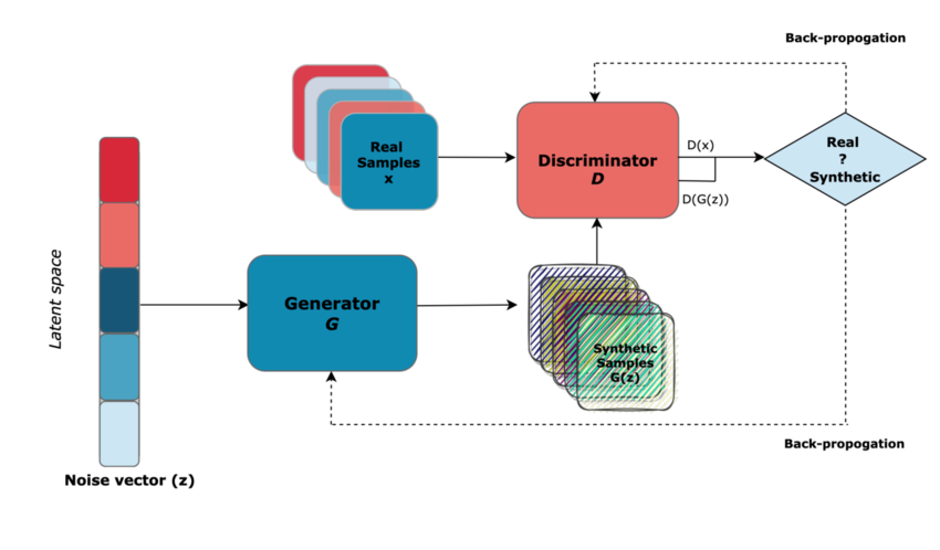
GANs — Structure and Components
Let’s now explore how these concepts come together in a GAN model. The key components of a GAN include the noise vector, the generator, and the discriminator.
The Generator: Generating Realistic Data
To generate synthetic data the generator uses a random noise vector as an input. In it’s bid to fool the discriminator, the generator aims to learn the distribution of the real data and produce synthetic data that cannot be distinguished from the real data. A problem here is that for the same input, it would always produce the same output (imagine an image generator that produced a realistic image but always the same image, that is not very useful). The random noise vector injects randomness into the process, providing diversity in the generated output.
The Discriminator: Discerning Real from Fake
The discriminator is like an art critic trained to differentiate between real and fake data. It’s role is to scrutinize the data it receives and assign a probability score of the work being real. If the synthetic data seems similar to the real data, the discriminator assigns a high probability, otherwise assign a low probability score.
Adversarial Training: A Dynamic Duel
The generator strives to learn to produce synthetic data that the discriminator can not differentiate from the real data. Simultaneously, the discriminator also learning and improving its ability to differentiate the real from the synthetic. This dynamic training process pushes both models to refine their skills. The two models are always competing with one another (hence why it is called Adversarial) and through this competition both models become excellent at their roles.
Implementing a GAN with Pytorch
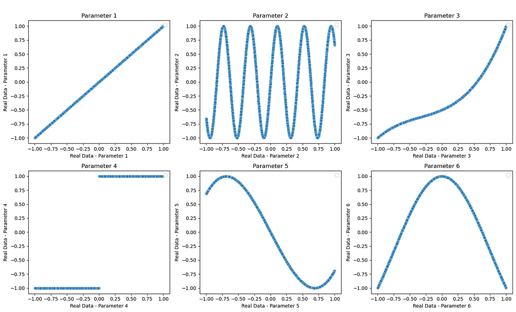
Let’s move forward by looking at an example of creating a GAN. In this example, we implement a model in pytorch that can generate synthetic data. For the training, we have a 6-parameters dataset with the following shapes (all parameters are plotted as a function of parameter 1). Each parameter has been deliberately chosen with a significantly different distribution and shape to increase the complexity of the dataset and mimic real-world data. However, it is worth mentioning that there is significant room for optimising both the discriminator and generator architectures but we won’t focus for this tutorial.
In this tutorial, I am assuming you already have an understanding normal ANN model architectures and python. I have provided comments in the code to help you follow the code.
Defining the GAN model components (Generator and Discriminator)
import torch
from torch import nn
from tqdm.auto import tqdm
from torch.utils.data import DataLoader
import matplotlib.pyplot as plt
import torch.nn.init as init
import pandas as pd
import numpy as np
from torch.utils.data import Dataset


# defining a single generation block function
def FC_Layer_blockGen(input_dim, output_dim):
    single_block = nn.Sequential(
        nn.Linear(input_dim, output_dim),

        nn.ReLU()
    )
    return single_block

# DEFINING THE GENERATOR
class Generator(nn.Module):
    def __init__(self, latent_dim, output_dim):
        super(Generator, self).__init__()
        self.model = nn.Sequential(
            nn.Linear(latent_dim, 256),
            nn.ReLU(),
            nn.Linear(256, 512),
            nn.ReLU(),
            nn.Linear(512, 512),
            nn.ReLU(),
            nn.Linear(512, output_dim),
            nn.Tanh()
        )

    def forward(self, x):
        return self.model(x)

#defining a single discriminattor block
def FC_Layer_BlockDisc(input_dim, output_dim):
    return nn.Sequential(
        nn.Linear(input_dim, output_dim),
        nn.ReLU(),
        nn.Dropout(0.4)
    )

# Defining the discriminator

class Discriminator(nn.Module):
    def __init__(self, input_dim):
        super(Discriminator, self).__init__()
        self.model = nn.Sequential(
            nn.Linear(input_dim, 512),
            nn.ReLU(),
            nn.Dropout(0.4),
            nn.Linear(512, 512),
            nn.ReLU(),
            nn.Dropout(0.4),
            nn.Linear(512, 256),
            nn.ReLU(),
            nn.Dropout(0.4),
            nn.Linear(256, 1),
            nn.Sigmoid()
        )

    def forward(self, x):
        return self.model(x)


#Defining training parameters
batch_size = 128
num_epochs = 500
lr = 0.0002
num_features = 6
latent_dim = 20

# MODEL INITIALIZATION
generator = Generator(noise_dim, num_features)
discriminator = Discriminator(num_features)

# LOSS FUNCTION AND OPTIMIZERS
criterion = nn.BCELoss()
gen_optimizer = torch.optim.Adam(generator.parameters(), lr=lr)
disc_optimizer = torch.optim.Adam(discriminator.parameters(), lr=lr)
Model Initialisation and Data Processing
# IMPORTING DATA
file_path = 'SamplingData7.xlsx'
data = pd.read_excel(file_path)
X = data.values
X_normalized = torch.FloatTensor((X - X.min(axis=0)) / (X.max(axis=0) - X.min(axis=0)) * 2 - 1)
real_data = X_normalized

#Creating a dataset

class MyDataset(Dataset):
    def __init__(self, dataframe):
        self.data = dataframe.values.astype(float)
        self.labels = dataframe.values.astype(float)

    def __len__(self):
        return len(self.data)

    def __getitem__(self, idx):
        sample = {
            'input': torch.tensor(self.data[idx]),
            'label': torch.tensor(self.labels[idx])
        }
        return sample

# Create an instance of the dataset
dataset = MyDataset(data)

# Create DataLoader
dataloader = DataLoader(dataset, batch_size=batch_size, shuffle=True, drop_last=True)

def weights_init(m):
    if isinstance(m, nn.Linear):
        init.xavier_uniform_(m.weight)
        if m.bias is not None:
            init.constant_(m.bias, 0)

pretrained = False
if pretrained:
    pre_dict = torch.load('pretrained_model.pth')
    generator.load_state_dict(pre_dict['generator'])
    discriminator.load_state_dict(pre_dict['discriminator'])
else:
    # Apply weight initialization
    generator = generator.apply(weights_init)
    discriminator = discriminator.apply(weights_init)
Model Training
model_save_freq = 100

latent_dim =20
for epoch in range(num_epochs):
    for batch in dataloader:
        real_data_batch = batch['input']
        # Train discriminator on real data
        real_labels = torch.FloatTensor(np.random.uniform(0.9, 1.0, (batch_size, 1)))
        disc_optimizer.zero_grad()
        output_real = discriminator(real_data_batch)
        loss_real = criterion(output_real, real_labels)
        loss_real.backward()

        # Train discriminator on generated data
        fake_labels = torch.FloatTensor(np.random.uniform(0, 0.1, (batch_size, 1)))
        noise = torch.FloatTensor(np.random.normal(0, 1, (batch_size, latent_dim)))
        generated_data = generator(noise)
        output_fake = discriminator(generated_data.detach())
        loss_fake = criterion(output_fake, fake_labels)
        loss_fake.backward()

        disc_optimizer.step()

        # Train generator
        valid_labels = torch.FloatTensor(np.random.uniform(0.9, 1.0, (batch_size, 1)))
        gen_optimizer.zero_grad()
        output_g = discriminator(generated_data)
        loss_g = criterion(output_g, valid_labels)
        loss_g.backward()
        gen_optimizer.step()

    # Print progress
    print(f"Epoch {epoch}, D Loss Real: {loss_real.item()}, D Loss Fake: {loss_fake.item()}, G Loss: {loss_g.item()}")
Evaluating and visualising the results
import seaborn as sns

# Generate synthetic data
synthetic_data = generator(torch.FloatTensor(np.random.normal(0, 1, (real_data.shape[0], noise_dim))))

# Plot the results
fig, axs = plt.subplots(2, 3, figsize=(12, 8))
fig.suptitle('Real and Synthetic Data Distributions', fontsize=16)

for i in range(2):
    for j in range(3):
        sns.histplot(synthetic_data[:, i * 3 + j].detach().numpy(), bins=50, alpha=0.5, label='Synthetic Data', ax=axs[i, j], color='blue')
        sns.histplot(real_data[:, i * 3 + j].numpy(), bins=50, alpha=0.5, label='Real Data', ax=axs[i, j], color='orange')
        axs[i, j].set_title(f'Parameter {i * 3 + j + 1}', fontsize=12)
        axs[i, j].set_xlabel('Value')
        axs[i, j].set_ylabel('Frequency')
        axs[i, j].legend()

plt.tight_layout(rect=[0, 0.03, 1, 0.95])
plt.show()


# Create a 2x3 grid of subplots
fig, axs = plt.subplots(2, 3, figsize=(15, 10))
fig.suptitle('Comparison of Real and Synthetic Data', fontsize=16)

# Define parameter names
param_names = ['Parameter 1', 'Parameter 2', 'Parameter 3', 'Parameter 4', 'Parameter 5', 'Parameter 6']

# Scatter plots for each parameter
for i in range(2):
    for j in range(3):
        param_index = i * 3 + j
        sns.scatterplot(real_data[:, 0].numpy(), real_data[:, param_index].numpy(), label='Real Data', alpha=0.5, ax=axs[i, j])
        sns.scatterplot(synthetic_data[:, 0].detach().numpy(), synthetic_data[:, param_index].detach().numpy(), label='Generated Data', alpha=0.5, ax=axs[i, j])
        axs[i, j].set_title(param_names[param_index], fontsize=12)
        axs[i, j].set_xlabel(f'Real Data - {param_names[param_index]}')
        axs[i, j].set_ylabel(f'Real Data - {param_names[param_index]}')
        axs[i, j].legend()

plt.tight_layout(rect=[0, 0.03, 1, 0.95])
plt.show()
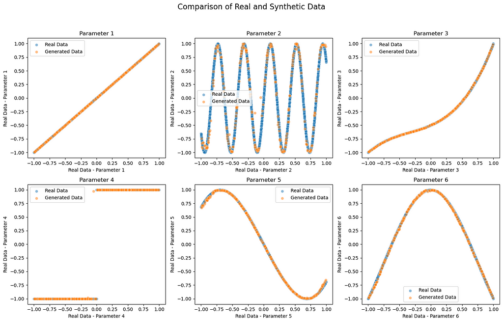
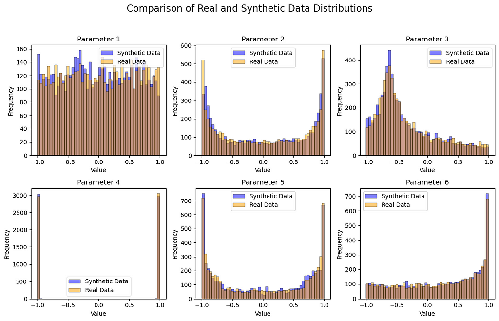
Despite the simplicity of our model, the distribution and mathematical shape of the synthetic data and real data look very similar! The training process and model architecture could be changed for improved accuracy, something we didn’t focus on here. This model could very easily be adjusted to produce synthetic data for other applications with larger number parameters and more complexity for real phyical systems. Thank you for taking the time to read, I hope you found this an informative read. There are so much one can do with GANs, it is a very exciting topic at the moment, definitely play around with this code to get the overall idea of GANs and then start experimenting with other ideas! best of luck!
Unless otherwise noted, all images are by the author
References
[1] Jaideep Pathak, Shashank Subramanian, Peter Harrington, Sanjeev Raja, Ashesh Chattopadhyay, Morteza Mardani, Thorsten Kurth, David Hall, Zongyi Li, Kamyar Azizzadenesheli, Pedram Hassanzadeh, Karthik Kashinath, Animashree Anandkumar. (2022). FourCastNet: A Global Data-driven High-resolution Weather Model using Adaptive Fourier Neural Operators. arXiv:2202.11214. https://doi.org/10.48550/arXiv.2202.11214
[2] Ghosheh, Ghadeer & Jin, Li & Zhu, Tingting. (2023). A Survey of Generative Adversarial Networks for Synthesizing Structured Electronic Health Records. ACM Computing Surveys. 10.1145/3636424.
Generative AI: Synthetic Data Generation with GANs using Pytorch was originally published in Towards Data Science on Medium, where people are continuing the conversation by highlighting and responding to this story.
Demystifying complexity: beyond images and language models
Generative Adversarial Networks (GANs) have become hugely popular for their abilities to generate both beautiful and realistic images, and language models (e.g. ChatGPT) that are increasingly rising in their use across every sector. These GAN models are arguably the reason AI/Machine learning have gotten the excitement (or fear) the world holds for the field right now; because it has shown everyone (especially those outside the field) the immense potential that machine learning holds. There are already a lot of resources on GANs models online but most of these focus on image generation. These image generation and language models require complex spatial or temporal intricacies which adds additional complexities that make it more challenging for readers to understand the true essence of GANs.
In an effort to remedy this and make GANs more accessible to a broader audience, in this short discussion and GAN model example, we’ll take a different and more practical approach that focuses on generating synthetic data of mathematical functions. Beyond being a simplification for learning purposes, synthetic data generation is becoming increasingly more important in its own right. Data is not only playing a central role in business decision-making but also there are an increasing number of uses where a data driven approach is becoming more popular than first principle models. An exciting example of this is weather forecast, the first principle model included simplified versions of the Navier-Stokes equation that was solved numerically (with significant computational costs I should add). However, recent attempts of weather forecast with deep learning (e.g. check out Nvidia’s FourCastNet [1]) have been very successful in capture weather patterns and once trained, it is easier and much faster to run.
Generative Models vs. Discriminative Models
In machine learning, it is important to understand the distinction between discriminative and generative models as they are the key components in a GAN. Let’s unravel these terms (very briefly):
Discriminative Models:
Discriminative models focus on classifying data into predefined classes for example classing images of dogs and cats into their respective classes. Rather than capturing the entire distribution, these models discern the boundaries that separate different classes. They output P(y|x) (probability of class, y given the input data, x) i.e. they answer the question of what category a given data point belongs to?
Generative Models:
Generative models aim to understand the underlying structure of the data. Unlike discriminative models that discern between classes, generative models learn the entire distribution of the data. These models output p(x|y) i.e. they answer the question of what is the likelihood of generating this specific data point given specified the class?
The interplay between these two models forms the very foundation of GANs.
GANs — Structure and Components
Let’s now explore how these concepts come together in a GAN model. The key components of a GAN include the noise vector, the generator, and the discriminator.
The Generator: Generating Realistic Data
To generate synthetic data the generator uses a random noise vector as an input. In it’s bid to fool the discriminator, the generator aims to learn the distribution of the real data and produce synthetic data that cannot be distinguished from the real data. A problem here is that for the same input, it would always produce the same output (imagine an image generator that produced a realistic image but always the same image, that is not very useful). The random noise vector injects randomness into the process, providing diversity in the generated output.
The Discriminator: Discerning Real from Fake
The discriminator is like an art critic trained to differentiate between real and fake data. It’s role is to scrutinize the data it receives and assign a probability score of the work being real. If the synthetic data seems similar to the real data, the discriminator assigns a high probability, otherwise assign a low probability score.
Adversarial Training: A Dynamic Duel
The generator strives to learn to produce synthetic data that the discriminator can not differentiate from the real data. Simultaneously, the discriminator also learning and improving its ability to differentiate the real from the synthetic. This dynamic training process pushes both models to refine their skills. The two models are always competing with one another (hence why it is called Adversarial) and through this competition both models become excellent at their roles.
Implementing a GAN with Pytorch
Let’s move forward by looking at an example of creating a GAN. In this example, we implement a model in pytorch that can generate synthetic data. For the training, we have a 6-parameters dataset with the following shapes (all parameters are plotted as a function of parameter 1). Each parameter has been deliberately chosen with a significantly different distribution and shape to increase the complexity of the dataset and mimic real-world data. However, it is worth mentioning that there is significant room for optimising both the discriminator and generator architectures but we won’t focus for this tutorial.
In this tutorial, I am assuming you already have an understanding normal ANN model architectures and python. I have provided comments in the code to help you follow the code.
Defining the GAN model components (Generator and Discriminator)
import torch
from torch import nn
from tqdm.auto import tqdm
from torch.utils.data import DataLoader
import matplotlib.pyplot as plt
import torch.nn.init as init
import pandas as pd
import numpy as np
from torch.utils.data import Dataset


# defining a single generation block function
def FC_Layer_blockGen(input_dim, output_dim):
    single_block = nn.Sequential(
        nn.Linear(input_dim, output_dim),

        nn.ReLU()
    )
    return single_block

# DEFINING THE GENERATOR
class Generator(nn.Module):
    def __init__(self, latent_dim, output_dim):
        super(Generator, self).__init__()
        self.model = nn.Sequential(
            nn.Linear(latent_dim, 256),
            nn.ReLU(),
            nn.Linear(256, 512),
            nn.ReLU(),
            nn.Linear(512, 512),
            nn.ReLU(),
            nn.Linear(512, output_dim),
            nn.Tanh()
        )

    def forward(self, x):
        return self.model(x)

#defining a single discriminattor block
def FC_Layer_BlockDisc(input_dim, output_dim):
    return nn.Sequential(
        nn.Linear(input_dim, output_dim),
        nn.ReLU(),
        nn.Dropout(0.4)
    )

# Defining the discriminator

class Discriminator(nn.Module):
    def __init__(self, input_dim):
        super(Discriminator, self).__init__()
        self.model = nn.Sequential(
            nn.Linear(input_dim, 512),
            nn.ReLU(),
            nn.Dropout(0.4),
            nn.Linear(512, 512),
            nn.ReLU(),
            nn.Dropout(0.4),
            nn.Linear(512, 256),
            nn.ReLU(),
            nn.Dropout(0.4),
            nn.Linear(256, 1),
            nn.Sigmoid()
        )

    def forward(self, x):
        return self.model(x)


#Defining training parameters
batch_size = 128
num_epochs = 500
lr = 0.0002
num_features = 6
latent_dim = 20

# MODEL INITIALIZATION
generator = Generator(noise_dim, num_features)
discriminator = Discriminator(num_features)

# LOSS FUNCTION AND OPTIMIZERS
criterion = nn.BCELoss()
gen_optimizer = torch.optim.Adam(generator.parameters(), lr=lr)
disc_optimizer = torch.optim.Adam(discriminator.parameters(), lr=lr)
Model Initialisation and Data Processing
# IMPORTING DATA
file_path = 'SamplingData7.xlsx'
data = pd.read_excel(file_path)
X = data.values
X_normalized = torch.FloatTensor((X - X.min(axis=0)) / (X.max(axis=0) - X.min(axis=0)) * 2 - 1)
real_data = X_normalized

#Creating a dataset

class MyDataset(Dataset):
    def __init__(self, dataframe):
        self.data = dataframe.values.astype(float)
        self.labels = dataframe.values.astype(float)

    def __len__(self):
        return len(self.data)

    def __getitem__(self, idx):
        sample = {
            'input': torch.tensor(self.data[idx]),
            'label': torch.tensor(self.labels[idx])
        }
        return sample

# Create an instance of the dataset
dataset = MyDataset(data)

# Create DataLoader
dataloader = DataLoader(dataset, batch_size=batch_size, shuffle=True, drop_last=True)

def weights_init(m):
    if isinstance(m, nn.Linear):
        init.xavier_uniform_(m.weight)
        if m.bias is not None:
            init.constant_(m.bias, 0)

pretrained = False
if pretrained:
    pre_dict = torch.load('pretrained_model.pth')
    generator.load_state_dict(pre_dict['generator'])
    discriminator.load_state_dict(pre_dict['discriminator'])
else:
    # Apply weight initialization
    generator = generator.apply(weights_init)
    discriminator = discriminator.apply(weights_init)
Model Training
model_save_freq = 100

latent_dim =20
for epoch in range(num_epochs):
    for batch in dataloader:
        real_data_batch = batch['input']
        # Train discriminator on real data
        real_labels = torch.FloatTensor(np.random.uniform(0.9, 1.0, (batch_size, 1)))
        disc_optimizer.zero_grad()
        output_real = discriminator(real_data_batch)
        loss_real = criterion(output_real, real_labels)
        loss_real.backward()

        # Train discriminator on generated data
        fake_labels = torch.FloatTensor(np.random.uniform(0, 0.1, (batch_size, 1)))
        noise = torch.FloatTensor(np.random.normal(0, 1, (batch_size, latent_dim)))
        generated_data = generator(noise)
        output_fake = discriminator(generated_data.detach())
        loss_fake = criterion(output_fake, fake_labels)
        loss_fake.backward()

        disc_optimizer.step()

        # Train generator
        valid_labels = torch.FloatTensor(np.random.uniform(0.9, 1.0, (batch_size, 1)))
        gen_optimizer.zero_grad()
        output_g = discriminator(generated_data)
        loss_g = criterion(output_g, valid_labels)
        loss_g.backward()
        gen_optimizer.step()

    # Print progress
    print(f"Epoch {epoch}, D Loss Real: {loss_real.item()}, D Loss Fake: {loss_fake.item()}, G Loss: {loss_g.item()}")
Evaluating and visualising the results
import seaborn as sns

# Generate synthetic data
synthetic_data = generator(torch.FloatTensor(np.random.normal(0, 1, (real_data.shape[0], noise_dim))))

# Plot the results
fig, axs = plt.subplots(2, 3, figsize=(12, 8))
fig.suptitle('Real and Synthetic Data Distributions', fontsize=16)

for i in range(2):
    for j in range(3):
        sns.histplot(synthetic_data[:, i * 3 + j].detach().numpy(), bins=50, alpha=0.5, label='Synthetic Data', ax=axs[i, j], color='blue')
        sns.histplot(real_data[:, i * 3 + j].numpy(), bins=50, alpha=0.5, label='Real Data', ax=axs[i, j], color='orange')
        axs[i, j].set_title(f'Parameter {i * 3 + j + 1}', fontsize=12)
        axs[i, j].set_xlabel('Value')
        axs[i, j].set_ylabel('Frequency')
        axs[i, j].legend()

plt.tight_layout(rect=[0, 0.03, 1, 0.95])
plt.show()


# Create a 2x3 grid of subplots
fig, axs = plt.subplots(2, 3, figsize=(15, 10))
fig.suptitle('Comparison of Real and Synthetic Data', fontsize=16)

# Define parameter names
param_names = ['Parameter 1', 'Parameter 2', 'Parameter 3', 'Parameter 4', 'Parameter 5', 'Parameter 6']

# Scatter plots for each parameter
for i in range(2):
    for j in range(3):
        param_index = i * 3 + j
        sns.scatterplot(real_data[:, 0].numpy(), real_data[:, param_index].numpy(), label='Real Data', alpha=0.5, ax=axs[i, j])
        sns.scatterplot(synthetic_data[:, 0].detach().numpy(), synthetic_data[:, param_index].detach().numpy(), label='Generated Data', alpha=0.5, ax=axs[i, j])
        axs[i, j].set_title(param_names[param_index], fontsize=12)
        axs[i, j].set_xlabel(f'Real Data - {param_names[param_index]}')
        axs[i, j].set_ylabel(f'Real Data - {param_names[param_index]}')
        axs[i, j].legend()

plt.tight_layout(rect=[0, 0.03, 1, 0.95])
plt.show()
Despite the simplicity of our model, the distribution and mathematical shape of the synthetic data and real data look very similar! The training process and model architecture could be changed for improved accuracy, something we didn’t focus on here. This model could very easily be adjusted to produce synthetic data for other applications with larger number parameters and more complexity for real phyical systems. Thank you for taking the time to read, I hope you found this an informative read. There are so much one can do with GANs, it is a very exciting topic at the moment, definitely play around with this code to get the overall idea of GANs and then start experimenting with other ideas! best of luck!
Unless otherwise noted, all images are by the author
References
[1] Jaideep Pathak, Shashank Subramanian, Peter Harrington, Sanjeev Raja, Ashesh Chattopadhyay, Morteza Mardani, Thorsten Kurth, David Hall, Zongyi Li, Kamyar Azizzadenesheli, Pedram Hassanzadeh, Karthik Kashinath, Animashree Anandkumar. (2022). FourCastNet: A Global Data-driven High-resolution Weather Model using Adaptive Fourier Neural Operators. arXiv:2202.11214. https://doi.org/10.48550/arXiv.2202.11214
[2] Ghosheh, Ghadeer & Jin, Li & Zhu, Tingting. (2023). A Survey of Generative Adversarial Networks for Synthesizing Structured Electronic Health Records. ACM Computing Surveys. 10.1145/3636424.
Generative AI: Synthetic Data Generation with GANs using Pytorch was originally published in Towards Data Science on Medium, where people are continuing the conversation by highlighting and responding to this story.
Denial of responsibility! Techno Blender is an automatic aggregator of the all world’s media. In each content, the hyperlink to the primary source is specified. All trademarks belong to their rightful owners, all materials to their authors. If you are the owner of the content and do not want us to publish your materials, please contact us by email – [email protected]. The content will be deleted within 24 hours.