
Graph Data Science for Tabular Data
Graph methods are more general than you may think
Graph data science methods are usually applied to data that has some inherent graphical nature, e.g., molecular structure data, transport network data, etc. However, graph methods can also be useful on data which does not display any obvious graphical structure, such as the tabular datasets used in machine learning tasks. In this article I will demonstrate simply and intuitively — without any mathematics or theory — that by representing tabular data as a graph we can open new possibilities for how to perform inference on this data.
To keep things simple, I will use the Credit Approval dataset below as an example. The objective is to predict the value of Approval based on the values of one or more of the other attributes. There are many classification algorithms that can be used to do this, but let’s explore how we might approach this using graphs.

Graph representation
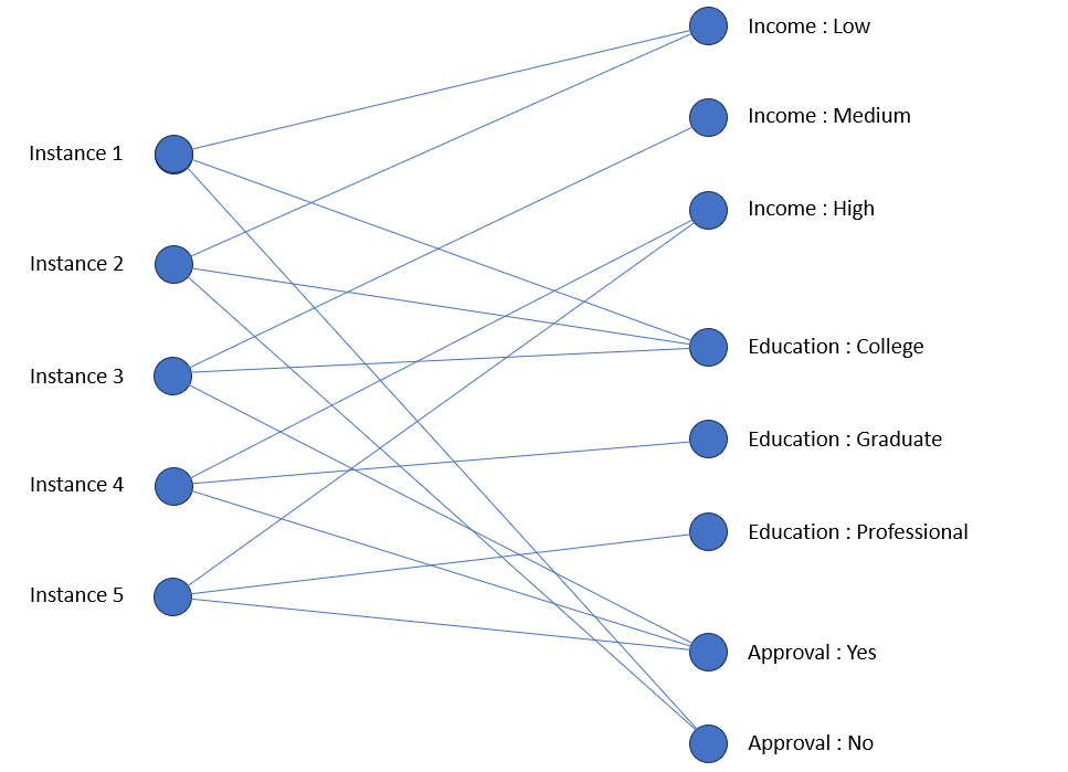
The first thing to consider is how to represent the data as a graph. We would like to capture the intuition that the greater the number of attribute values that are shared between two instances, the more similar are those instances. We will use one node to represent each instance (we refer to these nodes as instance nodes), and one node for each possible attribute value (these are attribute value nodes). The connections between instance nodes and attribute value nodes are bi-directional and reflect the information in the table. To keep things really simple, we will omit attributes Employment and History. Here is the graph.
Message Passing
Given attribute values for some new instance, there are several ways in which we might use graph methods to predict some unknown attribute value. We will use the notion of message passing. Here is the procedure we will use.
Message-passing procedure
Initiate a message with value 1 at the starting node, and let this node pass the message to each node to which it is connected. Let any node that receives a message then pass on the message (dilated by a factor k, where 0 <k<1) to each other node to which it is connected. Continue message passing until either a target node is reached (i.e., a node corresponding to the attribute whose value is being predicted), or there are no further nodes to pass the message to. Since a message cannot be passed back to a node from which it was received the process is guaranteed to terminate.
When message passing has completed, each node in the graph will have received zero or more messages of varying value. Sum these values for each node belonging to the target attribute, and then normalize these (sum) values so that they themselves sum to 1. Interpret the normalized values as probabilities. These probabilities can then be used to either predict the unknown attribute value or to impute a random value drawn from the distribution. Dilating message values at each pass reflects the intuition that longer paths should contribute less to the probability estimate than shorter paths.
Example 1
Suppose that we wish to predict the value of Approval given that Income is Low. The arrows on the graph below illustrate the operation of the message-passing procedure, with the thickness of each arrow representing the message value (dilated by factor k = 0.5 at every hop).
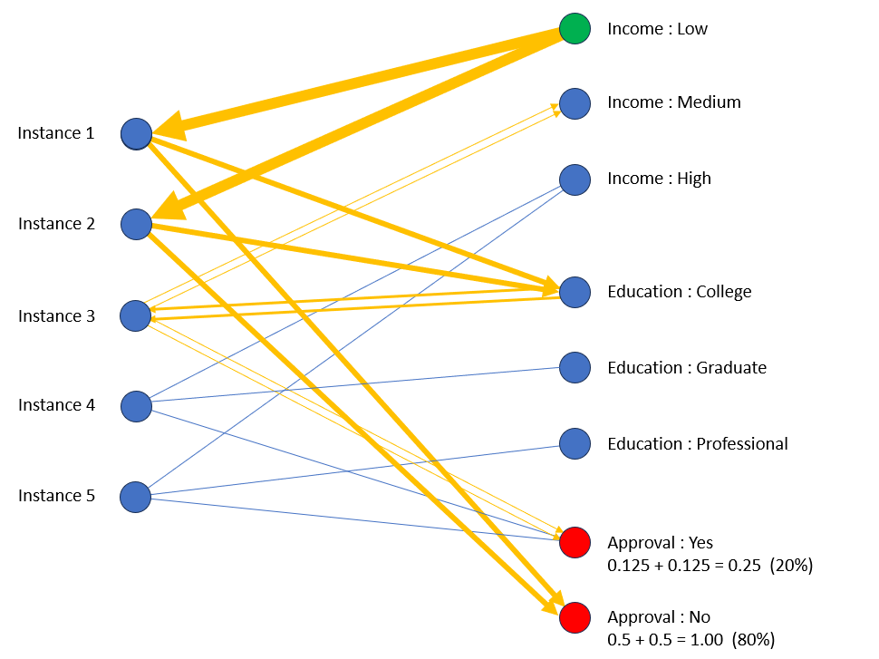
The message is initiated at node Income:Low (colored green). This node passes messages of value 1 to both Instance 1 and Instance 2, which then each pass the message (with a dilated value of 0.5) to nodes Education:College and Approval:No. Note that since Education:College receives messages from both Instance 1 and Instance 2, it must pass each of these messages to Instance 3, with a dilated value of 0.25. The numbers at each node of the target variable show the sum of message values received and (in parentheses) the normalized values as percentages. We have the following probabilities for Approval, conditional on Income is Low:
- Prob (Approval is ‘Yes’ | Income is Low) = 20%
- Prob (Approval is ‘No’ | Income is Low) = 80%
These probabilities are different to what we would have obtained from a count-based prediction from the table. Since two of the five instances have Income Low, and both of these have Approval No, a count-based prediction would lead to a probability of 100% for Approval No.
The message-passing procedure has taken into account that the attribute value Education College, possessed by Instances 1 and 2, is also possessed by Instance 3, which has Approval Yes, thus contributing to the total message value received at node Approval:Yes. If we had incorporated the additional attributes Employment and History in our graph, this would likely have further increased the number of paths connecting the start node to the target nodes, thereby utilizing additional contextual information, and improving the estimate of the probability distribution.
Example 2
The message-passing procedure can also be used when conditioning on more than one attribute. In such a case we simply initiate a message at each of the nodes corresponding to the attribute values we are conditioning on and follow the same procedure from each. The graph below shows the result of predicting the value of Approval given Income is Low and Education is Graduate. The sequence of messages originating from each starting node are shown in different colors.
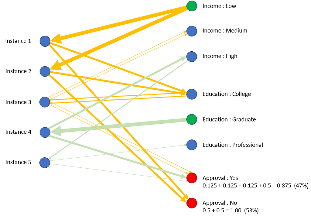
Instance 4 has Education value Graduate, and therefore contributes to the sum of message values received at node Approval:Yes. A further contribution to Approval:Yes is made by Instance 5, which shares Income High with Instance 4.
[Note: in each of these examples we have used Approval as our target variable; however, we could have estimated the probability distributions for Income or Education in exactly the same way].
These examples demonstrate that the simple notion of message passing (a fundamentally graph-based operation), coupled with an appropriate graph representation, allows us to perform inference of a general and flexible nature. Specifically, it can be used to estimate the probability distribution of ANY attribute, conditional on the values of ONE or MORE attributes.
The inference procedure is somewhat ad hoc, devised to make our argument as simply as possible. There are many variations that we could have used. The crucial point is that graph methods enable us to utilize the rich network of relationships between instances in a way that is difficult to capture using vector-based approaches. We could of course attempt to express the message-passing procedure in terms of vectors (i.e., with reference to the table as opposed to the graph) but this would be convoluted and cumbersome. The simplicity and elegance of the graph-based approach arise from the natural pairing of the graph representation and the inference procedure.
There is another interesting observation that we can make from our examples. In the analysis above we did not make any reference to the sum of message values received at the instance nodes (i.e., the nodes along the left-hand side of the graphs). Let’s see what these values can show us. In Example 1, at the completion of message passing the sum of message values at Instance nodes 1 to 5 are respectively 1.0, 1.0, 0.5, 0.0 and 0.0. Normalizing these values to sum to 1 results in 40%, 40%, 20%, 0% and 0%. The first two instances have Approval No, and the sum of their normalized values is 80%. The last three instances have Approval Yes, and the sum of their normalized values is 20%. But these are just the probabilities we obtained for attribute Approval in the original analysis. (You can verify the same for Example 2). This is no coincidence. The sum of message values at an instance node can be interpreted as representing the similarity of that instance to the attribute values we are conditioning on. Thus, the inference procedure can be considered a form of weighted nearest neighbor, in which the similarity measure is implicit in the message-passing procedure.
The UNCRi framework
At Skanalytix we have developed a graph-based computational framework named Unified Numerical/Categorical Representation and Inference (UNCRi). The framework combines a unique graph-based data representation with a flexible inference procedure and can be used to estimate and sample from the conditional distribution of any categorical or numeric variable. It can be applied to tasks such as classification and regression, missing value imputation, anomaly detection, and synthetic data generation from either the full joint distribution or some conditional distribution. The framework is robust to extremities in the data: categorical variables can range from binary to high cardinality; numerical variables can be multi-modal, highly skewed and of arbitrary scale; and the missing-value ratio can be high. You can find out more about UNCRi at http://skanalytix.com. (UNCRi code is closed source).
Conclusion
The Pattern Recognition and Machine Learning disciplines have from the outset been dominated by methods that operate on vectors. Vectors have been so ubiquitous that it can be difficult to conceive of any other approach. Graph methods provide a powerful and flexible alternative. When applied to tabular data, graph methods can be used to not only predict the value of an attribute or impute an attribute with a random value drawn from its estimated distribution, but — by using the chain rule of probability — to generate entire synthetic datasets of instances distributed in the same way as the source data. And all of this from one graph and one inference procedure! While in this article we have considered only categorical variables, it is possible to extend these ideas to datasets containing a mix of numeric and categorical attributes.
Graph Data Science for Tabular Data was originally published in Towards Data Science on Medium, where people are continuing the conversation by highlighting and responding to this story.
Graph methods are more general than you may think

Graph data science methods are usually applied to data that has some inherent graphical nature, e.g., molecular structure data, transport network data, etc. However, graph methods can also be useful on data which does not display any obvious graphical structure, such as the tabular datasets used in machine learning tasks. In this article I will demonstrate simply and intuitively — without any mathematics or theory — that by representing tabular data as a graph we can open new possibilities for how to perform inference on this data.
To keep things simple, I will use the Credit Approval dataset below as an example. The objective is to predict the value of Approval based on the values of one or more of the other attributes. There are many classification algorithms that can be used to do this, but let’s explore how we might approach this using graphs.
Graph representation
The first thing to consider is how to represent the data as a graph. We would like to capture the intuition that the greater the number of attribute values that are shared between two instances, the more similar are those instances. We will use one node to represent each instance (we refer to these nodes as instance nodes), and one node for each possible attribute value (these are attribute value nodes). The connections between instance nodes and attribute value nodes are bi-directional and reflect the information in the table. To keep things really simple, we will omit attributes Employment and History. Here is the graph.
Message Passing
Given attribute values for some new instance, there are several ways in which we might use graph methods to predict some unknown attribute value. We will use the notion of message passing. Here is the procedure we will use.
Message-passing procedure
Initiate a message with value 1 at the starting node, and let this node pass the message to each node to which it is connected. Let any node that receives a message then pass on the message (dilated by a factor k, where 0 <k<1) to each other node to which it is connected. Continue message passing until either a target node is reached (i.e., a node corresponding to the attribute whose value is being predicted), or there are no further nodes to pass the message to. Since a message cannot be passed back to a node from which it was received the process is guaranteed to terminate.
When message passing has completed, each node in the graph will have received zero or more messages of varying value. Sum these values for each node belonging to the target attribute, and then normalize these (sum) values so that they themselves sum to 1. Interpret the normalized values as probabilities. These probabilities can then be used to either predict the unknown attribute value or to impute a random value drawn from the distribution. Dilating message values at each pass reflects the intuition that longer paths should contribute less to the probability estimate than shorter paths.
Example 1
Suppose that we wish to predict the value of Approval given that Income is Low. The arrows on the graph below illustrate the operation of the message-passing procedure, with the thickness of each arrow representing the message value (dilated by factor k = 0.5 at every hop).
The message is initiated at node Income:Low (colored green). This node passes messages of value 1 to both Instance 1 and Instance 2, which then each pass the message (with a dilated value of 0.5) to nodes Education:College and Approval:No. Note that since Education:College receives messages from both Instance 1 and Instance 2, it must pass each of these messages to Instance 3, with a dilated value of 0.25. The numbers at each node of the target variable show the sum of message values received and (in parentheses) the normalized values as percentages. We have the following probabilities for Approval, conditional on Income is Low:
- Prob (Approval is ‘Yes’ | Income is Low) = 20%
- Prob (Approval is ‘No’ | Income is Low) = 80%
These probabilities are different to what we would have obtained from a count-based prediction from the table. Since two of the five instances have Income Low, and both of these have Approval No, a count-based prediction would lead to a probability of 100% for Approval No.
The message-passing procedure has taken into account that the attribute value Education College, possessed by Instances 1 and 2, is also possessed by Instance 3, which has Approval Yes, thus contributing to the total message value received at node Approval:Yes. If we had incorporated the additional attributes Employment and History in our graph, this would likely have further increased the number of paths connecting the start node to the target nodes, thereby utilizing additional contextual information, and improving the estimate of the probability distribution.
Example 2
The message-passing procedure can also be used when conditioning on more than one attribute. In such a case we simply initiate a message at each of the nodes corresponding to the attribute values we are conditioning on and follow the same procedure from each. The graph below shows the result of predicting the value of Approval given Income is Low and Education is Graduate. The sequence of messages originating from each starting node are shown in different colors.
Instance 4 has Education value Graduate, and therefore contributes to the sum of message values received at node Approval:Yes. A further contribution to Approval:Yes is made by Instance 5, which shares Income High with Instance 4.
[Note: in each of these examples we have used Approval as our target variable; however, we could have estimated the probability distributions for Income or Education in exactly the same way].
These examples demonstrate that the simple notion of message passing (a fundamentally graph-based operation), coupled with an appropriate graph representation, allows us to perform inference of a general and flexible nature. Specifically, it can be used to estimate the probability distribution of ANY attribute, conditional on the values of ONE or MORE attributes.
The inference procedure is somewhat ad hoc, devised to make our argument as simply as possible. There are many variations that we could have used. The crucial point is that graph methods enable us to utilize the rich network of relationships between instances in a way that is difficult to capture using vector-based approaches. We could of course attempt to express the message-passing procedure in terms of vectors (i.e., with reference to the table as opposed to the graph) but this would be convoluted and cumbersome. The simplicity and elegance of the graph-based approach arise from the natural pairing of the graph representation and the inference procedure.
There is another interesting observation that we can make from our examples. In the analysis above we did not make any reference to the sum of message values received at the instance nodes (i.e., the nodes along the left-hand side of the graphs). Let’s see what these values can show us. In Example 1, at the completion of message passing the sum of message values at Instance nodes 1 to 5 are respectively 1.0, 1.0, 0.5, 0.0 and 0.0. Normalizing these values to sum to 1 results in 40%, 40%, 20%, 0% and 0%. The first two instances have Approval No, and the sum of their normalized values is 80%. The last three instances have Approval Yes, and the sum of their normalized values is 20%. But these are just the probabilities we obtained for attribute Approval in the original analysis. (You can verify the same for Example 2). This is no coincidence. The sum of message values at an instance node can be interpreted as representing the similarity of that instance to the attribute values we are conditioning on. Thus, the inference procedure can be considered a form of weighted nearest neighbor, in which the similarity measure is implicit in the message-passing procedure.
The UNCRi framework
At Skanalytix we have developed a graph-based computational framework named Unified Numerical/Categorical Representation and Inference (UNCRi). The framework combines a unique graph-based data representation with a flexible inference procedure and can be used to estimate and sample from the conditional distribution of any categorical or numeric variable. It can be applied to tasks such as classification and regression, missing value imputation, anomaly detection, and synthetic data generation from either the full joint distribution or some conditional distribution. The framework is robust to extremities in the data: categorical variables can range from binary to high cardinality; numerical variables can be multi-modal, highly skewed and of arbitrary scale; and the missing-value ratio can be high. You can find out more about UNCRi at http://skanalytix.com. (UNCRi code is closed source).
Conclusion
The Pattern Recognition and Machine Learning disciplines have from the outset been dominated by methods that operate on vectors. Vectors have been so ubiquitous that it can be difficult to conceive of any other approach. Graph methods provide a powerful and flexible alternative. When applied to tabular data, graph methods can be used to not only predict the value of an attribute or impute an attribute with a random value drawn from its estimated distribution, but — by using the chain rule of probability — to generate entire synthetic datasets of instances distributed in the same way as the source data. And all of this from one graph and one inference procedure! While in this article we have considered only categorical variables, it is possible to extend these ideas to datasets containing a mix of numeric and categorical attributes.
Graph Data Science for Tabular Data was originally published in Towards Data Science on Medium, where people are continuing the conversation by highlighting and responding to this story.
Denial of responsibility! Techno Blender is an automatic aggregator of the all world’s media. In each content, the hyperlink to the primary source is specified. All trademarks belong to their rightful owners, all materials to their authors. If you are the owner of the content and do not want us to publish your materials, please contact us by email – [email protected]. The content will be deleted within 24 hours.