
How Autoencoders Outperform PCA in Dimensionality Reduction | by Rukshan Pramoditha | Aug, 2022
Applications of Autoencoders
Dimensionality reduction with autoencoders using non-linear data
There are so many practical applications of autoencoders. Dimensionality reduction is one of them.
There are so many techniques for dimensionality reduction. Autoencoders (AEs) and Principal Component Analysis (PCA) are popular among them.
PCA is not suitable for dimensionality reduction in non-linear data. In contrast, autoencoders work really well with non-linear data in dimensionality reduction.
At the end of this article, you’ll be able to
- Use Autoencoders to reduce the dimensionality of the input data
- Use PCA to reduce the dimensionality of the input data
- Compare the performance of PCA and Autoencoders in dimensionality reduction
- See how Autoencoders outperform PCA in dimensionality reduction
- Learn key differences between PCA and Autoencoders
- Learn when to use which method for dimensionality reduction
I recommend you to read the following articles as the prerequisites for this article.
First, we’ll perform dimensionality reduction on the MNIST data (see dataset Citation at the end) using PCA and compare the output with the original MNIST data.
- Step 1: Acquire and prepare the MNIST dataset.
- Step 2: Apply PCA with only two components. The original dimensionality of the input data is 784.
- Step 3: Visualize compressed MNIST digits after PCA.
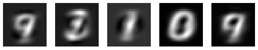
- Step 4: Compare the PCA output with the original MNIST digits.

As you can see in the two outputs, the MNIST digits are not clearly visible after applying PCA. This is because we only kept two components that do not capture much of the patterns in the input data.
- Step 5: Visualize test data using the two principal components.
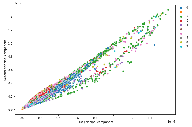
All the digits do not have clear separate clusters. It means that the PCA model with only two components cannot clearly distinguish between the nine digits in the test data.
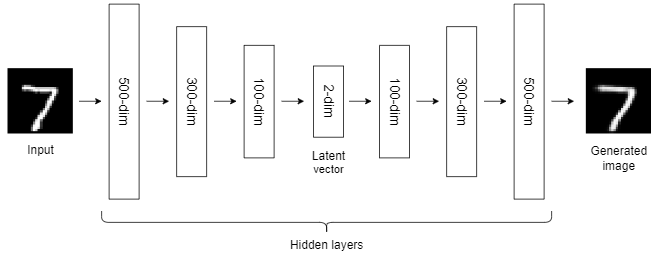
Now, we’ll build a deep autoencoder to apply dimensionality reduction to the same MNIST data. We also keep the dimensionality of the latent vector two-dimensional so that it is easy to compare the output with the previous output returned by PCA.
- Step 1: Acquire and prepare the MNIST dataset as previously.
- Step 2: Define the autoencoder architecture.
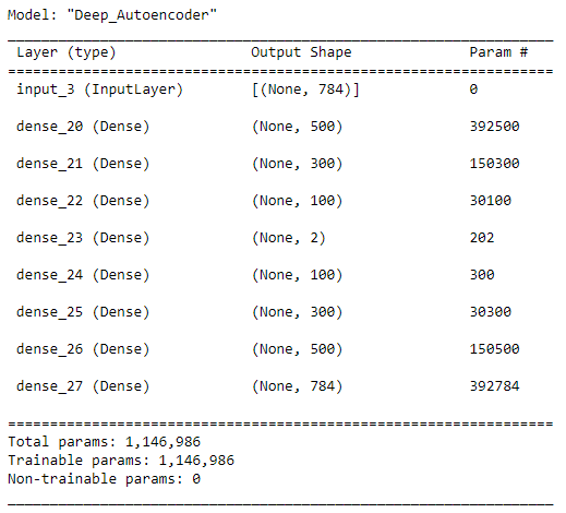
There are over one million parameters in the network. So, that will require a lot of computational power to train this model. If you use a traditional CPU for this, it will take a lot of time to complete the training process. It is better to use a powerful NVIDIA GPU or Colab free GPU to speed up the training process by a factor of 10 or 20.
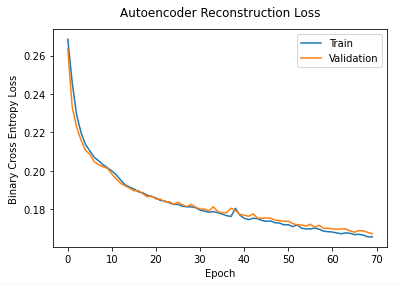
- Step 3: Compile, train and monitor the loss function.
- Step 4: Visualize compressed MNIST digits after autoencoding.
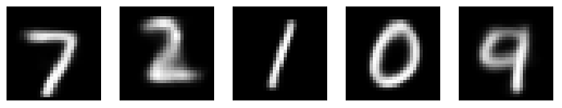
The autoencoder output is much better than the PCA output. This is because autoencoders can learn complex non-linear patterns in the data. In contrast, PCA can only learn linear patterns in the data.
- Step 5: Visualize test data in the latent space to see how the autoencoder model is capable of distinguishing between the nine digits in the test data.
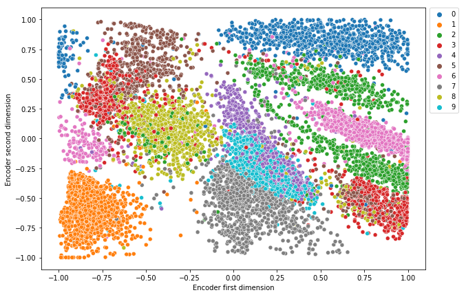
Most of the digits have clear separate clusters. It means that the autoencoder model can clearly distinguish between most digits in the test data. Some digits overlap, for example, there is an overlap between digits 4 and 9. It means that the autoencoder model cannot clearly distinguish between digits 4 and 9.
- Step 6 (Optional): Use the same autoencoder model but without using any activation function in the hidden layers,
activation=Nonein each hidden layer. You’ll get the following output.

This output is even worse than the PCA output. I used this experiment to show you the importance of activation functions in neural networks. Activation functions are needed in the hidden layers of neural networks to learn non-linear relationships in the data. Without activation functions in the hidden layers, neural networks are giant linear models and behave even worse than general machine learning algorithms! So, you need to use the right activation function for neural networks.
- Architecture: PCA is a general machine learning algorithm. It uses Eigendecomposition or Singular Value Decomposition (SVD) of the covariance matrix of the input data to perform dimensionality reduction. In contrast, Autoencoder is a neural network-based architecture that is more complex than PCA.
- Size of the input dataset: PCA generally works well with small datasets. Because Autoencoder is a neural network, it requires a lot of data compared to PCA. So, it is better to use Autoencoders with very large datasets.
- Linear vs non-linear: PCA is a linear dimensionality reduction technique. It can only learn linear relationships in the data. In contrast, Autoencoder is a non-linear dimensionality reduction technique that can also learn complex non-linear relationships in the data. That’s why the Autoencoder output is much better than the PCA output in our example as there are complex non-linear patterns in the MNSIT data.
- Usage: PCA is only used for dimensionality reduction. But, Autoencoders are not limited to dimensionality reduction. They have other practical applications such as image denoising, image colonization, super-resolution, image compression, feature extraction, image generation, watermark removal, etc.
- Computational resources: Autoencoders require more computational resources than PCA.
- Training time: PCA takes less time to run as compared to autoencoders.
- Interpretability: Autoencoders are less interpretable than PCA.
You can build different autoencoder architectures by trying different values for the following hyperparameters. After doing, let me know the results in the comment section.
- Number of layers
- Number of nodes in each layer
- Dimension of the latent vector
- Type of activation function in the hidden layers
- Type of optimizer
- Learning rate
- Number of epochs
- Batch size
Consider the following diagram that consists of all the outputs we obtained before.
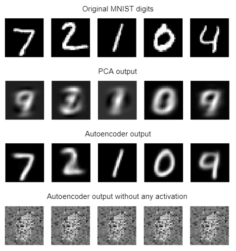
- The first row represents the original MNIST digits.
- The second row represents the output returned by PCA with only two components. The digits are not clearly visible.
- The third row represents the output returned by the autoencoder with a two-dimensional latent vector that is much better than the PCA output. The digits are clearly visible now. The reason is that the autoencoder has learned complex non-linear patterns in the MNIST data.
- The last row represents the output returned by the autoencoder without any activation function in the hidden layers. That output is even worse than the PCA output. I included this to show you the importance of activation functions in neural networks. Activation functions are needed in the hidden layers of neural networks to learn non-linear relationships in the data. Without activation functions in the hidden layers, neural networks are giant linear models and behave even worse than general machine learning algorithms!
Applications of Autoencoders
Dimensionality reduction with autoencoders using non-linear data

There are so many practical applications of autoencoders. Dimensionality reduction is one of them.
There are so many techniques for dimensionality reduction. Autoencoders (AEs) and Principal Component Analysis (PCA) are popular among them.
PCA is not suitable for dimensionality reduction in non-linear data. In contrast, autoencoders work really well with non-linear data in dimensionality reduction.
At the end of this article, you’ll be able to
- Use Autoencoders to reduce the dimensionality of the input data
- Use PCA to reduce the dimensionality of the input data
- Compare the performance of PCA and Autoencoders in dimensionality reduction
- See how Autoencoders outperform PCA in dimensionality reduction
- Learn key differences between PCA and Autoencoders
- Learn when to use which method for dimensionality reduction
I recommend you to read the following articles as the prerequisites for this article.
First, we’ll perform dimensionality reduction on the MNIST data (see dataset Citation at the end) using PCA and compare the output with the original MNIST data.
- Step 1: Acquire and prepare the MNIST dataset.
- Step 2: Apply PCA with only two components. The original dimensionality of the input data is 784.
- Step 3: Visualize compressed MNIST digits after PCA.
- Step 4: Compare the PCA output with the original MNIST digits.
As you can see in the two outputs, the MNIST digits are not clearly visible after applying PCA. This is because we only kept two components that do not capture much of the patterns in the input data.
- Step 5: Visualize test data using the two principal components.
All the digits do not have clear separate clusters. It means that the PCA model with only two components cannot clearly distinguish between the nine digits in the test data.
Now, we’ll build a deep autoencoder to apply dimensionality reduction to the same MNIST data. We also keep the dimensionality of the latent vector two-dimensional so that it is easy to compare the output with the previous output returned by PCA.
- Step 1: Acquire and prepare the MNIST dataset as previously.
- Step 2: Define the autoencoder architecture.
There are over one million parameters in the network. So, that will require a lot of computational power to train this model. If you use a traditional CPU for this, it will take a lot of time to complete the training process. It is better to use a powerful NVIDIA GPU or Colab free GPU to speed up the training process by a factor of 10 or 20.
- Step 3: Compile, train and monitor the loss function.
- Step 4: Visualize compressed MNIST digits after autoencoding.
The autoencoder output is much better than the PCA output. This is because autoencoders can learn complex non-linear patterns in the data. In contrast, PCA can only learn linear patterns in the data.
- Step 5: Visualize test data in the latent space to see how the autoencoder model is capable of distinguishing between the nine digits in the test data.
Most of the digits have clear separate clusters. It means that the autoencoder model can clearly distinguish between most digits in the test data. Some digits overlap, for example, there is an overlap between digits 4 and 9. It means that the autoencoder model cannot clearly distinguish between digits 4 and 9.
- Step 6 (Optional): Use the same autoencoder model but without using any activation function in the hidden layers,
activation=Nonein each hidden layer. You’ll get the following output.
This output is even worse than the PCA output. I used this experiment to show you the importance of activation functions in neural networks. Activation functions are needed in the hidden layers of neural networks to learn non-linear relationships in the data. Without activation functions in the hidden layers, neural networks are giant linear models and behave even worse than general machine learning algorithms! So, you need to use the right activation function for neural networks.
- Architecture: PCA is a general machine learning algorithm. It uses Eigendecomposition or Singular Value Decomposition (SVD) of the covariance matrix of the input data to perform dimensionality reduction. In contrast, Autoencoder is a neural network-based architecture that is more complex than PCA.
- Size of the input dataset: PCA generally works well with small datasets. Because Autoencoder is a neural network, it requires a lot of data compared to PCA. So, it is better to use Autoencoders with very large datasets.
- Linear vs non-linear: PCA is a linear dimensionality reduction technique. It can only learn linear relationships in the data. In contrast, Autoencoder is a non-linear dimensionality reduction technique that can also learn complex non-linear relationships in the data. That’s why the Autoencoder output is much better than the PCA output in our example as there are complex non-linear patterns in the MNSIT data.
- Usage: PCA is only used for dimensionality reduction. But, Autoencoders are not limited to dimensionality reduction. They have other practical applications such as image denoising, image colonization, super-resolution, image compression, feature extraction, image generation, watermark removal, etc.
- Computational resources: Autoencoders require more computational resources than PCA.
- Training time: PCA takes less time to run as compared to autoencoders.
- Interpretability: Autoencoders are less interpretable than PCA.
You can build different autoencoder architectures by trying different values for the following hyperparameters. After doing, let me know the results in the comment section.
- Number of layers
- Number of nodes in each layer
- Dimension of the latent vector
- Type of activation function in the hidden layers
- Type of optimizer
- Learning rate
- Number of epochs
- Batch size
Consider the following diagram that consists of all the outputs we obtained before.
- The first row represents the original MNIST digits.
- The second row represents the output returned by PCA with only two components. The digits are not clearly visible.
- The third row represents the output returned by the autoencoder with a two-dimensional latent vector that is much better than the PCA output. The digits are clearly visible now. The reason is that the autoencoder has learned complex non-linear patterns in the MNIST data.
- The last row represents the output returned by the autoencoder without any activation function in the hidden layers. That output is even worse than the PCA output. I included this to show you the importance of activation functions in neural networks. Activation functions are needed in the hidden layers of neural networks to learn non-linear relationships in the data. Without activation functions in the hidden layers, neural networks are giant linear models and behave even worse than general machine learning algorithms!
Denial of responsibility! Techno Blender is an automatic aggregator of the all world’s media. In each content, the hyperlink to the primary source is specified. All trademarks belong to their rightful owners, all materials to their authors. If you are the owner of the content and do not want us to publish your materials, please contact us by email – [email protected]. The content will be deleted within 24 hours.