
How Midjourney and Other Diffusion Models Create Images from Random Noise
Colossal hype ensues whenever there’s progress or even the slightest shift in the world of machine learning (ML). When it comes to AI, the craze always ends up growing out of proportion and insane claims invariably follow. You’ve probably noticed this recently as more people are beginning to use Midjourney, ChatGPT, Copilot, and so on.
The truth about these systems, however, is always more prosaic. Machine learning is mathematical, and the real implications of the ML models are not nearly as profound as some bloggers would have you believe. They could be beneficial and, in some cases, transform large portions of workflows in specific areas, but only if the user, whether an organization or an individual, has a sufficient understanding of their inner workings, limitations, capabilities, and potential.
This article hopes to shed some light on how diffusion models work, such as the highly popular Midjourney, DALL-E 2, and Stable Diffusion, and particularly how they are trained. This post includes mathematical expressions, but it also describes what each variable represents in an accessible manner.
Forward Diffusion
All diffusion models, including Midjourney (although we don’t have a paper describing it yet), are multi-element neural networks that create images from randomness. Initially, they are trained to gradually turn pictures into noise. This method establishes a Markov chain* consisting of timesteps, in which the image goes through a series of transformations and evolves from an initial pure state at t=0 to total noise at t=T, the final step.
*A Markov chain is a sequence of variables in which the state of one variable depends only on the state of the previous variable.
The number of timesteps, which can range from a few hundred to a thousand or more, and the noise levels to be applied at each step must be predetermined; this is known as the noising schedule. Mathematically, this noising or the forward diffusion process is denoted as:
q(xt|xt-1) = N(xt; √(1-βt) xt-1, βtI)
q(x0) is our real distribution and q(xt∣xt−1) is the forward diffusion process in which xt is always conditioned on xt-1. The symbol N stands for Gaussian or normal distribution, which is defined by the mean μ and variance σ^2. In this case, the mean is represented by √(1-βt)xt-1, where βt is our variance. The noise is sampled from a normal distribution at each step ϵ∼N(0,I) and the variance schedule is predetermined.
In simpler terms, we have a normal distribution over the current step where the mean is represented by √(1-βt) times the image of the previous step xt-1. In addition to this rescaling, we also add a small amount of noise βtI to the pic on each iteration. Think of β as a tiny, positive scalar value, for example, 0.001, and it is small on purpose.
So, this is what’s done at each time step. But, we can also define a joint distribution for all the samples that will be generated in the xt, x2, x3, …, xT sequence. It will look like this:
q(x1:T|x0) = ∏t=1:T q(xt|xt-1)
As you can see, this joint distribution is represented by the product ∏ of conditional distributions q(xt|xt-1), created at timesteps 1 through T, and then given the initial image x0.
OK, But Can We Skip Links in the Chain to Generate Any xt Without Going Through All the Preceding Steps?
Yes, we can.
This is possible because we use a simple Gaussian kernel to diffuse the data. To do this, we compute the scalar value αt, which is equal to 1 – βt, and we define the variable ᾱt as the product of αs from t1 to t. The forward diffusion variances βt are essential to the process. They can be learned by reparameterization or held constant as hyperparameters, but they are always designed to make ᾱt approach 0 on the final step T. This ensures that the diffused data has a normal distribution, which is crucial for the reverse generative process.
After we have the kernel, we can just sample any xt, because:
xt = √ᾱt x0 + √(1 – ᾱt)ε, where ε (noise) is derived from a normal distribution with a mean of 0 and an Identity covariance matrix I.
In lay terms, if we need xt, which represents a random step in our Markov chain, we can generate it with no problem given that x0, ᾱt, and the noise term ε are available.
Generative Process
Let’s now delve into the reverse process, where the model generates new samples. The first thing to understand is that we cannot compute the denoising distribution q(xt-1|xt) directly, as it would require knowing the distribution of all the images in the dataset. Although, we can use Bayes’ rule to show that this distribution is proportional to the product of the marginal data distribution q(xt-1) and our diffusion kernel at step t – q(xt|xt-1):
q(xt-1|xt) ∝ q(xt-1) q(xt|xt-1)
But, the product and the distribution would still be intractable. So, what we need to do is to approximate the conditional probability distribution. Luckily, we can do so by using a normal distribution since the noise injections βt were small during the forward process.
We can represent our approximation of the conditional probability distribution as pθ(xt−1∣xt), where θ is the model’s parameters that are iteratively optimized through gradient descent.
When we remember that the end of our Markov chain is a normal distribution, we can assume that the backward process will also be Gaussian. Therefore, it must be parameterized by the mean μθ and variance Σθ, which our neural network will have to compute.
This is the process parameterization: pθ(xt−1∣xt)=N(xt−1;μθ(xt,t),Σθ(xt,t))
In the original paper, Denoising Diffusion Probabilistic Models, researchers found that fixing the variance Σθ(xt, t) = σ2tI was an optimal choice in terms of sample quality. In particular, they found that fixing the variance to β gives roughly the same results as fixing it to βt, since when we add diffusion steps to the process, β and βt remain close to each other, therefore the mean, not variance, is actually what determines the distributions.
Note: in the paper “Improved Denoising Diffusion Probabilistic Models,” which came out a bit later, the researchers did parameterize the variance too. It helped improve the log-likelihood but did not increase sample efficiency.
So How Do We Determine the Objective Function to Derive the Mean?
Since q and pθ can be viewed as a variational autoencoder, a model that approximates the data distribution by encoding data into a latent space* and then back into the input space, we can use the variational upper bound (ELBO) objective function to train it. It minimizes the negative log-likelihood with respect to x0. Here, the variational lower bound is the sum of losses on each time step, and each term of the loss is the KL divergence** between the two Gaussian distributions.
*Latent space is a compressed space in which the input features are represented by separate dimensions; it helps the models easily find patterns and similarities between data objects.
**KL divergence is a measurement of the distance between two distributions. It basically tells you how much information you would lose if you approximate the target distribution with a model distribution.
As you recall, we can sample xt at any noise level that is conditioned on x0. Because of q(xt|x0) = N(xt;√(α̅t)x0, (1-α̅t)I), we’re able to add and scale noise to x0 in order to get to any xt. Additionally, since α̅t are functions of βt, the predetermined variance, we can easily optimize the random terms of the loss function L during training.
Another important benefit of this property is that we can turn our network into a noise predictor instead of a mean predictor. Specifically, the mean can be reparameterized to make the model approximate added noise at step t using εθ(xt, t) in the KL divergence terms. Like:
μθ(xt, t) = (1/√αt) (xt – (βt/√(1-α¯t)) εθ(xt, t))
Finally, we arrive at this equation for the objective loss function Lt (at a random time step, given that the noise is sampled from the random distribution N (0, I)):
||ε – εθ(xt, t)||^2 = ||ε – εθ(√α¯t x0 + √(1-α¯t)ε, t)||^2
Where x0 is the uncorrupted image, ϵ is the pure noise sampled at time t, and εθ(xt, t) is the predicted noise obtained by passing the approximated value xt through our neural network, which is parametrized by θ.
The network is optimized by the mean squared error between predicted and true noise. By minimizing the distance between true and predicted errors, we teach the model to make progressively more accurate approximations.
So, in summary, here’s a sequence of training steps that gives us models, such as Midhjourney and Stable Diffusion, that can generate images from pure noise.
From the original paper.
Colossal hype ensues whenever there’s progress or even the slightest shift in the world of machine learning (ML). When it comes to AI, the craze always ends up growing out of proportion and insane claims invariably follow. You’ve probably noticed this recently as more people are beginning to use Midjourney, ChatGPT, Copilot, and so on.
The truth about these systems, however, is always more prosaic. Machine learning is mathematical, and the real implications of the ML models are not nearly as profound as some bloggers would have you believe. They could be beneficial and, in some cases, transform large portions of workflows in specific areas, but only if the user, whether an organization or an individual, has a sufficient understanding of their inner workings, limitations, capabilities, and potential.
This article hopes to shed some light on how diffusion models work, such as the highly popular Midjourney, DALL-E 2, and Stable Diffusion, and particularly how they are trained. This post includes mathematical expressions, but it also describes what each variable represents in an accessible manner.
Forward Diffusion
All diffusion models, including Midjourney (although we don’t have a paper describing it yet), are multi-element neural networks that create images from randomness. Initially, they are trained to gradually turn pictures into noise. This method establishes a Markov chain* consisting of timesteps, in which the image goes through a series of transformations and evolves from an initial pure state at t=0 to total noise at t=T, the final step.
*A Markov chain is a sequence of variables in which the state of one variable depends only on the state of the previous variable.
The number of timesteps, which can range from a few hundred to a thousand or more, and the noise levels to be applied at each step must be predetermined; this is known as the noising schedule. Mathematically, this noising or the forward diffusion process is denoted as:
q(xt|xt-1) = N(xt; √(1-βt) xt-1, βtI)
q(x0) is our real distribution and q(xt∣xt−1) is the forward diffusion process in which xt is always conditioned on xt-1. The symbol N stands for Gaussian or normal distribution, which is defined by the mean μ and variance σ^2. In this case, the mean is represented by √(1-βt)xt-1, where βt is our variance. The noise is sampled from a normal distribution at each step ϵ∼N(0,I) and the variance schedule is predetermined.
In simpler terms, we have a normal distribution over the current step where the mean is represented by √(1-βt) times the image of the previous step xt-1. In addition to this rescaling, we also add a small amount of noise βtI to the pic on each iteration. Think of β as a tiny, positive scalar value, for example, 0.001, and it is small on purpose.
So, this is what’s done at each time step. But, we can also define a joint distribution for all the samples that will be generated in the xt, x2, x3, …, xT sequence. It will look like this:
q(x1:T|x0) = ∏t=1:T q(xt|xt-1)
As you can see, this joint distribution is represented by the product ∏ of conditional distributions q(xt|xt-1), created at timesteps 1 through T, and then given the initial image x0.
OK, But Can We Skip Links in the Chain to Generate Any xt Without Going Through All the Preceding Steps?
Yes, we can.
This is possible because we use a simple Gaussian kernel to diffuse the data. To do this, we compute the scalar value αt, which is equal to 1 – βt, and we define the variable ᾱt as the product of αs from t1 to t. The forward diffusion variances βt are essential to the process. They can be learned by reparameterization or held constant as hyperparameters, but they are always designed to make ᾱt approach 0 on the final step T. This ensures that the diffused data has a normal distribution, which is crucial for the reverse generative process.
After we have the kernel, we can just sample any xt, because:
xt = √ᾱt x0 + √(1 – ᾱt)ε, where ε (noise) is derived from a normal distribution with a mean of 0 and an Identity covariance matrix I.
In lay terms, if we need xt, which represents a random step in our Markov chain, we can generate it with no problem given that x0, ᾱt, and the noise term ε are available.
Generative Process
Let’s now delve into the reverse process, where the model generates new samples. The first thing to understand is that we cannot compute the denoising distribution q(xt-1|xt) directly, as it would require knowing the distribution of all the images in the dataset. Although, we can use Bayes’ rule to show that this distribution is proportional to the product of the marginal data distribution q(xt-1) and our diffusion kernel at step t – q(xt|xt-1):
q(xt-1|xt) ∝ q(xt-1) q(xt|xt-1)
But, the product and the distribution would still be intractable. So, what we need to do is to approximate the conditional probability distribution. Luckily, we can do so by using a normal distribution since the noise injections βt were small during the forward process.
We can represent our approximation of the conditional probability distribution as pθ(xt−1∣xt), where θ is the model’s parameters that are iteratively optimized through gradient descent.
When we remember that the end of our Markov chain is a normal distribution, we can assume that the backward process will also be Gaussian. Therefore, it must be parameterized by the mean μθ and variance Σθ, which our neural network will have to compute.
This is the process parameterization: pθ(xt−1∣xt)=N(xt−1;μθ(xt,t),Σθ(xt,t))
In the original paper, Denoising Diffusion Probabilistic Models, researchers found that fixing the variance Σθ(xt, t) = σ2tI was an optimal choice in terms of sample quality. In particular, they found that fixing the variance to β gives roughly the same results as fixing it to βt, since when we add diffusion steps to the process, β and βt remain close to each other, therefore the mean, not variance, is actually what determines the distributions.
Note: in the paper “Improved Denoising Diffusion Probabilistic Models,” which came out a bit later, the researchers did parameterize the variance too. It helped improve the log-likelihood but did not increase sample efficiency.
So How Do We Determine the Objective Function to Derive the Mean?
Since q and pθ can be viewed as a variational autoencoder, a model that approximates the data distribution by encoding data into a latent space* and then back into the input space, we can use the variational upper bound (ELBO) objective function to train it. It minimizes the negative log-likelihood with respect to x0. Here, the variational lower bound is the sum of losses on each time step, and each term of the loss is the KL divergence** between the two Gaussian distributions.
*Latent space is a compressed space in which the input features are represented by separate dimensions; it helps the models easily find patterns and similarities between data objects.
**KL divergence is a measurement of the distance between two distributions. It basically tells you how much information you would lose if you approximate the target distribution with a model distribution.
As you recall, we can sample xt at any noise level that is conditioned on x0. Because of q(xt|x0) = N(xt;√(α̅t)x0, (1-α̅t)I), we’re able to add and scale noise to x0 in order to get to any xt. Additionally, since α̅t are functions of βt, the predetermined variance, we can easily optimize the random terms of the loss function L during training.
Another important benefit of this property is that we can turn our network into a noise predictor instead of a mean predictor. Specifically, the mean can be reparameterized to make the model approximate added noise at step t using εθ(xt, t) in the KL divergence terms. Like:
μθ(xt, t) = (1/√αt) (xt – (βt/√(1-α¯t)) εθ(xt, t))
Finally, we arrive at this equation for the objective loss function Lt (at a random time step, given that the noise is sampled from the random distribution N (0, I)):
||ε – εθ(xt, t)||^2 = ||ε – εθ(√α¯t x0 + √(1-α¯t)ε, t)||^2
Where x0 is the uncorrupted image, ϵ is the pure noise sampled at time t, and εθ(xt, t) is the predicted noise obtained by passing the approximated value xt through our neural network, which is parametrized by θ.
The network is optimized by the mean squared error between predicted and true noise. By minimizing the distance between true and predicted errors, we teach the model to make progressively more accurate approximations.
So, in summary, here’s a sequence of training steps that gives us models, such as Midhjourney and Stable Diffusion, that can generate images from pure noise.
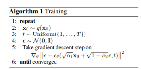
From the original paper.
Denial of responsibility! Techno Blender is an automatic aggregator of the all world’s media. In each content, the hyperlink to the primary source is specified. All trademarks belong to their rightful owners, all materials to their authors. If you are the owner of the content and do not want us to publish your materials, please contact us by email – [email protected]. The content will be deleted within 24 hours.