
How to Create a Graph Neural Network in Python | by Tiago Toledo Jr. | Jul, 2022
Creating a GNN with Pytorch Geometric and OGB
Deep learning has opened a whole new world of possibilities for making predictions on non-structured data. Today it is common to use Convolutional Neural Networks (CNNs) on image data, Recurrent Neural Networks (RNNs) for text, and so on.
Over the last years, a new exciting class of neural networks has emerged: Graph Neural Networks (GNNs). As the name implies, this network class focuses on working with graph data.
In this post, you will learn the basics of how a Graph Neural Network works and how one can start implementing it in Python using the Pytorch Geometric (PyG) library and the Open Graph Benchmark (OGB) library.
The notebook with the codes for this post is available on my Github and Kaggle.
GNNs started getting popular with the introduction of the Graph Convolutional Network (GCN) [1] which borrowed some concepts from the CNNs to the graph world. The main idea from this kind of network, also known as Message-Passing Framework, became the golden standard for many years in the area, and it is this the concept we will explore here.
The Message-Passing framework states that, for every node in our graph, we will do two things:
- Aggregate the information from its neighbors
- Update the node information with the information from its previous layer and its neighbor aggregation
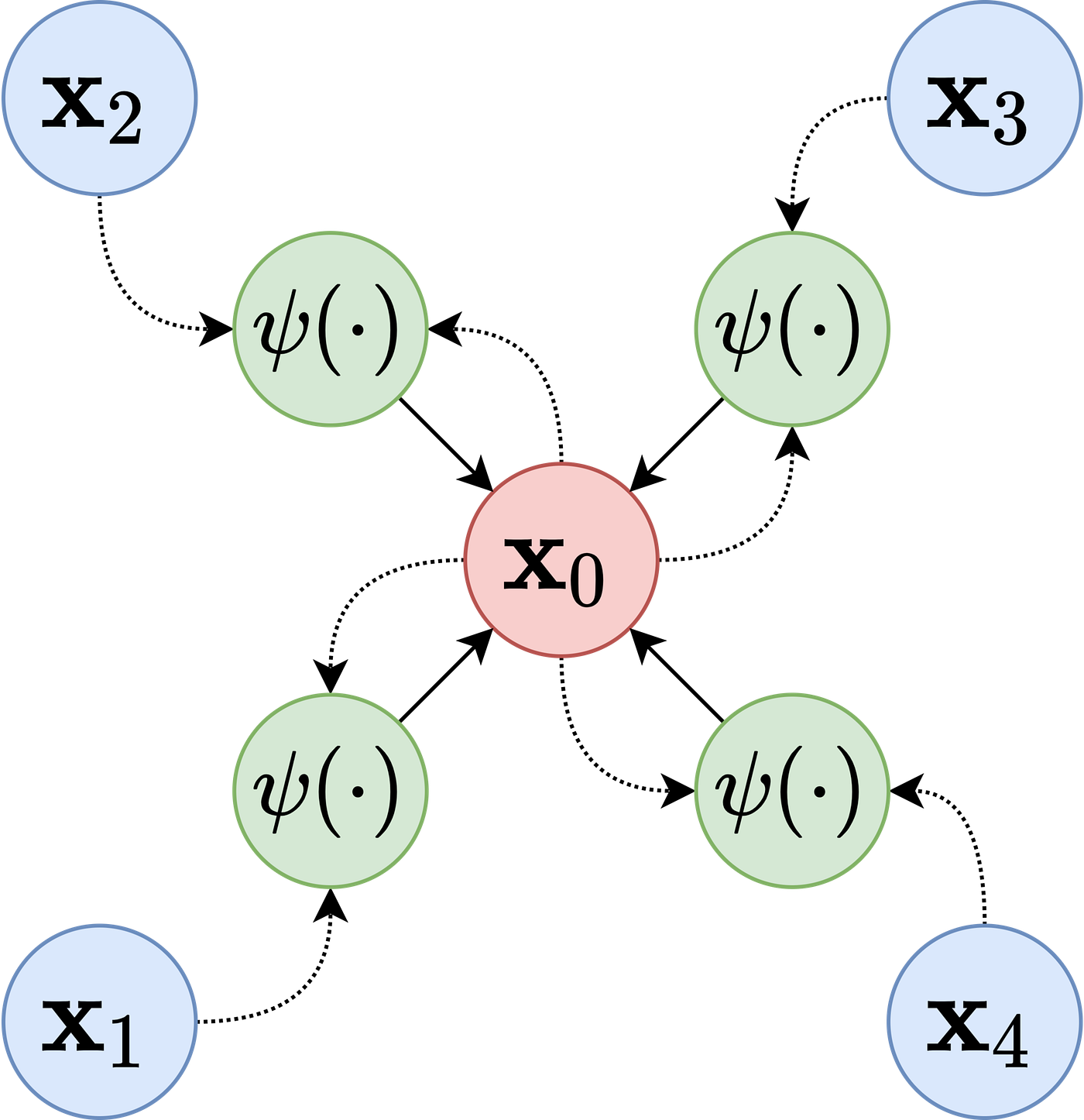
Image 1 shows how this general framework works. Many architectures developed after GCN focused on defining the best way of aggregating and updating the data.
The PyG is an extension for the Pytorch library which allows us to quickly implement new GNNs architectures using already established layers from research.
The OGB [2] was developed as a way of improving the quality of the research on the area since it provides curated graphs to be used and also a standard way of evaluating the results from a given architecture, making so that the comparison between proposals is fairer.
The idea of using those two libraries together is that one can more easily propose an architecture and does not have to worry about the data obtention and the evaluation mechanism.
First, let’s install the required libraries. Notice here that you must have PyTorch installed:
pip install ogb
pip install torch_geometric
Now, let’s import the required methods and libraries:
import os
import torch
import torch.nn.functional as Ffrom tqdm import tqdm
from torch_geometric.loader import NeighborLoader
from torch.optim.lr_scheduler import ReduceLROnPlateau
from torch_geometric.nn import MessagePassing, SAGEConv
from ogb.nodeproppred import Evaluator, PygNodePropPredDataset
The first step will be downloading the dataset from the OGB. We will use the ogbn-arxiv network in which each node is a Computer Science paper on the arxiv and each directed edge represents that a paper cited another. The task is to classify each node into a paper class.
Downloading it is as simple as:
target_dataset = 'ogbn-arxiv'# This will download the ogbn-arxiv to the 'networks' folder
dataset = PygNodePropPredDataset(name=target_dataset, root='networks')
The dataset variable is an instance of a class named PygNodePropPredDataset() which is specific to the OGB. To access the dataset as a Data class that can be used on the Pytorch Geometric we can just do:
data = dataset[0]
If we take a look at this variable, we will see something like:
Data(num_nodes=169343, edge_index=[2, 1166243], x=[169343, 128], node_year=[169343, 1], y=[169343, 1])
We have the number of nodes, the adjacency list, the feature vector for the network, the year for each node, and the target label.
This network already comes with a split set for training, validation, and testing. This is provided by the OGB as a way of improving reproducibility and the quality of research on this network. We can extract this with:
split_idx = dataset.get_idx_split() train_idx = split_idx['train']
valid_idx = split_idx['valid']
test_idx = split_idx['test']
Now, we will define two Data Loaders to use during our training. The first one will load only nodes from the training set and the second one will load all nodes on the network.
We will use the NeighborLoader from the Pytorch Geometric. This data loader samples a given number of neighbors for every node. This is a way of avoiding the explosion of RAM and computation time for nodes that have thousands of nodes. For this tutorial, we will use 30 neighbors per node on the training loader.
train_loader = NeighborLoader(data, input_nodes=train_idx,
shuffle=True, num_workers=os.cpu_count() - 2,
batch_size=1024, num_neighbors=[30] * 2)total_loader = NeighborLoader(data, input_nodes=None, num_neighbors=[-1],
batch_size=4096, shuffle=False,
num_workers=os.cpu_count() - 2)
Notice that we shuffle the training data loader but not the total loader. Also, the number of neighbors for the training loader is defined as the number per layer of the network. Since we are going to use a two-layer network here, we set it to the list with two values 30.
Now it is time to create our GNN architecture. For anyone familiar with Pytorch this should not be too scary.
We will use the SAGE layers. These layers were defined in a very good paper [3] that introduced the idea of neighbor sampling. The Pytorch Geometric library already has this layer implemented for us.
So, as with every PyTorch architecture, we must define a class with the layers we are going to use:
class SAGE(torch.nn.Module):
def __init__(self, in_channels,
hidden_channels, out_channels,
n_layers=2):super(SAGE, self).__init__()
self.layers = torch.nn.ModuleList()
self.n_layers = n_layers
self.layers_bn = torch.nn.ModuleList() if n_layers == 1:
self.layers.append(SAGEConv(in_channels, out_channels, normalize=False))
elif n_layers == 2:
self.layers.append(SAGEConv(in_channels, hidden_channels, normalize=False))
self.layers_bn.append(torch.nn.BatchNorm1d(hidden_channels))
self.layers.append(SAGEConv(hidden_channels, out_channels, normalize=False))
else:
self.layers.append(SAGEConv(in_channels, hidden_channels, normalize=False))
self.layers_bn.append(torch.nn.BatchNorm1d(hidden_channels)) for _ in range(n_layers - 2):
self.layers.append(SAGEConv(hidden_channels, hidden_channels, normalize=False))
self.layers_bn.append(torch.nn.BatchNorm1d(hidden_channels))self.layers.append(SAGEConv(hidden_channels, out_channels, normalize=False))
for layer in self.layers:
def forward(self, x, edge_index):
layer.reset_parameters()
if len(self.layers) > 1:
looper = self.layers[:-1]
else:
looper = self.layersfor i, layer in enumerate(looper):
x = layer(x, edge_index)
try:
x = self.layers_bn[i](x)
except Exception as e:
abs(1)
finally:
x = F.relu(x)
x = F.dropout(x, p=0.5, training=self.training)if len(self.layers) > 1:
return F.log_softmax(x, dim=-1), torch.var(x)
x = self.layers[-1](x, edge_index)def inference(self, total_loader, device):
xs = []
var_ = []
for batch in total_loader:
out, var = self.forward(batch.x.to(device), batch.edge_index.to(device))
out = out[:batch.batch_size]
xs.append(out.cpu())
var_.append(var.item())out_all = torch.cat(xs, dim=0)
return out_all, var_
Let’s break this down step by step:
- We must define the number of in_channels of the network, this will be the number of features in our dataset. The out_channels is going to be the number of classes we are trying to predict. The hidden channels parameter is a value we can define ourselves that represents the number of hidden units.
- We can set the number of layers of the network. For each hidden layer, we add a Batch Normalization layer and then we reset the parameters for every layer.
- The forward method runs a single iteration of a forward pass. It will get the feature vector and the adjacency list and pass it to the SAGE Layer and then pass the result to the Batch Normalization layer. We also apply a ReLU non-linearity and a dropout layer for regularization purposes.
- Finally, the inference method will generate a prediction for every node in the dataset. We will use it for validation purposes.
Now, let’s define some parameters of our model:
device = torch.device('cuda' if torch.cuda.is_available() else 'cpu')model = SAGE(data.x.shape[1], 256, dataset.num_classes, n_layers=2)
model.to(device)
epochs = 100
optimizer = torch.optim.Adam(model.parameters(), lr=0.03)
scheduler = ReduceLROnPlateau(optimizer, 'max', patience=7)
Now, we shall make the test function that will validate all of our predictions:
def test(model, device):
evaluator = Evaluator(name=target_dataset)
model.eval()
out, var = model.inference(total_loader, device)    y_true = data.y.cpu()
y_pred = out.argmax(dim=-1, keepdim=True)    train_acc = evaluator.eval({
'y_true': y_true[split_idx['train']],
'y_pred': y_pred[split_idx['train']],
})['acc']
val_acc = evaluator.eval({
'y_true': y_true[split_idx['valid']],
'y_pred': y_pred[split_idx['valid']],
})['acc']
test_acc = evaluator.eval({
'y_true': y_true[split_idx['test']],
'y_pred': y_pred[split_idx['test']],
})['acc']return train_acc, val_acc, test_acc, torch.mean(torch.Tensor(var))
In this function, we instantiate a Validator class from the OGB. This class will take care of the validation of our model for every split we retrieved previously. This way, we will see the score for the train, validation, and test sets on each epoch.
Finally, let’s create our training loop:
for epoch in range(1, epochs):
model.train()    pbar = tqdm(total=train_idx.size(0))
pbar.set_description(f'Epoch {epoch:02d}')    total_loss = total_correct = 0    for batch in train_loader:
batch_size = batch.batch_size
optimizer.zero_grad()        out, _ = model(batch.x.to(device), batch.edge_index.to(device))
out = out[:batch_size]        batch_y = batch.y[:batch_size].to(device)
batch_y = torch.reshape(batch_y, (-1,))        loss = F.nll_loss(out, batch_y)
loss.backward()
optimizer.step()        total_loss += float(loss)
total_correct += int(out.argmax(dim=-1).eq(batch_y).sum())
pbar.update(batch.batch_size)    pbar.close()    loss = total_loss / len(train_loader)
approx_acc = total_correct / train_idx.size(0)    train_acc, val_acc, test_acc, var = test(model, device)print(f'Train: {train_acc:.4f}, Val: {val_acc:.4f}, Test: {test_acc:.4f}, Var: {var:.4f}')
This loop will train our GNN for 100 epochs and will early stop it if our validation score does not grow for seven epochs straight.
GNNs are a fascinating class of Neural Networks. Today we already have several tools to help us develop this kind of solution. As you can see, one using Pytorch Geometric and OGB can easily implement a GNN for some graphs.
[1] Kipf, Thomas & Welling, Max. (2016). Semi-Supervised Classification with Graph Convolutional Networks.
[2] Hu, W., Fey, M., Zitnik, M., Dong, Y., Ren, H., Liu, B., Catasta, M., & Leskovec, J. (2020). Open Graph Benchmark: Datasets for Machine Learning on Graphs. arXiv preprint arXiv:2005.00687.
[3] Hamilton, William & Ying, Rex & Leskovec, Jure. (2017). Inductive Representation Learning on Large Graphs.
Creating a GNN with Pytorch Geometric and OGB
Deep learning has opened a whole new world of possibilities for making predictions on non-structured data. Today it is common to use Convolutional Neural Networks (CNNs) on image data, Recurrent Neural Networks (RNNs) for text, and so on.
Over the last years, a new exciting class of neural networks has emerged: Graph Neural Networks (GNNs). As the name implies, this network class focuses on working with graph data.
In this post, you will learn the basics of how a Graph Neural Network works and how one can start implementing it in Python using the Pytorch Geometric (PyG) library and the Open Graph Benchmark (OGB) library.
The notebook with the codes for this post is available on my Github and Kaggle.
GNNs started getting popular with the introduction of the Graph Convolutional Network (GCN) [1] which borrowed some concepts from the CNNs to the graph world. The main idea from this kind of network, also known as Message-Passing Framework, became the golden standard for many years in the area, and it is this the concept we will explore here.
The Message-Passing framework states that, for every node in our graph, we will do two things:
- Aggregate the information from its neighbors
- Update the node information with the information from its previous layer and its neighbor aggregation
Image 1 shows how this general framework works. Many architectures developed after GCN focused on defining the best way of aggregating and updating the data.
The PyG is an extension for the Pytorch library which allows us to quickly implement new GNNs architectures using already established layers from research.
The OGB [2] was developed as a way of improving the quality of the research on the area since it provides curated graphs to be used and also a standard way of evaluating the results from a given architecture, making so that the comparison between proposals is fairer.
The idea of using those two libraries together is that one can more easily propose an architecture and does not have to worry about the data obtention and the evaluation mechanism.
First, let’s install the required libraries. Notice here that you must have PyTorch installed:
pip install ogb
pip install torch_geometric
Now, let’s import the required methods and libraries:
import os
import torch
import torch.nn.functional as Ffrom tqdm import tqdm
from torch_geometric.loader import NeighborLoader
from torch.optim.lr_scheduler import ReduceLROnPlateau
from torch_geometric.nn import MessagePassing, SAGEConv
from ogb.nodeproppred import Evaluator, PygNodePropPredDataset
The first step will be downloading the dataset from the OGB. We will use the ogbn-arxiv network in which each node is a Computer Science paper on the arxiv and each directed edge represents that a paper cited another. The task is to classify each node into a paper class.
Downloading it is as simple as:
target_dataset = 'ogbn-arxiv'# This will download the ogbn-arxiv to the 'networks' folder
dataset = PygNodePropPredDataset(name=target_dataset, root='networks')
The dataset variable is an instance of a class named PygNodePropPredDataset() which is specific to the OGB. To access the dataset as a Data class that can be used on the Pytorch Geometric we can just do:
data = dataset[0]
If we take a look at this variable, we will see something like:
Data(num_nodes=169343, edge_index=[2, 1166243], x=[169343, 128], node_year=[169343, 1], y=[169343, 1])
We have the number of nodes, the adjacency list, the feature vector for the network, the year for each node, and the target label.
This network already comes with a split set for training, validation, and testing. This is provided by the OGB as a way of improving reproducibility and the quality of research on this network. We can extract this with:
split_idx = dataset.get_idx_split() train_idx = split_idx['train']
valid_idx = split_idx['valid']
test_idx = split_idx['test']
Now, we will define two Data Loaders to use during our training. The first one will load only nodes from the training set and the second one will load all nodes on the network.
We will use the NeighborLoader from the Pytorch Geometric. This data loader samples a given number of neighbors for every node. This is a way of avoiding the explosion of RAM and computation time for nodes that have thousands of nodes. For this tutorial, we will use 30 neighbors per node on the training loader.
train_loader = NeighborLoader(data, input_nodes=train_idx,
shuffle=True, num_workers=os.cpu_count() - 2,
batch_size=1024, num_neighbors=[30] * 2)total_loader = NeighborLoader(data, input_nodes=None, num_neighbors=[-1],
batch_size=4096, shuffle=False,
num_workers=os.cpu_count() - 2)
Notice that we shuffle the training data loader but not the total loader. Also, the number of neighbors for the training loader is defined as the number per layer of the network. Since we are going to use a two-layer network here, we set it to the list with two values 30.
Now it is time to create our GNN architecture. For anyone familiar with Pytorch this should not be too scary.
We will use the SAGE layers. These layers were defined in a very good paper [3] that introduced the idea of neighbor sampling. The Pytorch Geometric library already has this layer implemented for us.
So, as with every PyTorch architecture, we must define a class with the layers we are going to use:
class SAGE(torch.nn.Module):
def __init__(self, in_channels,
hidden_channels, out_channels,
n_layers=2):super(SAGE, self).__init__()
self.layers = torch.nn.ModuleList()
self.n_layers = n_layers
self.layers_bn = torch.nn.ModuleList() if n_layers == 1:
self.layers.append(SAGEConv(in_channels, out_channels, normalize=False))
elif n_layers == 2:
self.layers.append(SAGEConv(in_channels, hidden_channels, normalize=False))
self.layers_bn.append(torch.nn.BatchNorm1d(hidden_channels))
self.layers.append(SAGEConv(hidden_channels, out_channels, normalize=False))
else:
self.layers.append(SAGEConv(in_channels, hidden_channels, normalize=False))
self.layers_bn.append(torch.nn.BatchNorm1d(hidden_channels)) for _ in range(n_layers - 2):
self.layers.append(SAGEConv(hidden_channels, hidden_channels, normalize=False))
self.layers_bn.append(torch.nn.BatchNorm1d(hidden_channels))self.layers.append(SAGEConv(hidden_channels, out_channels, normalize=False))
for layer in self.layers:
def forward(self, x, edge_index):
layer.reset_parameters()
if len(self.layers) > 1:
looper = self.layers[:-1]
else:
looper = self.layersfor i, layer in enumerate(looper):
x = layer(x, edge_index)
try:
x = self.layers_bn[i](x)
except Exception as e:
abs(1)
finally:
x = F.relu(x)
x = F.dropout(x, p=0.5, training=self.training)if len(self.layers) > 1:
return F.log_softmax(x, dim=-1), torch.var(x)
x = self.layers[-1](x, edge_index)def inference(self, total_loader, device):
xs = []
var_ = []
for batch in total_loader:
out, var = self.forward(batch.x.to(device), batch.edge_index.to(device))
out = out[:batch.batch_size]
xs.append(out.cpu())
var_.append(var.item())out_all = torch.cat(xs, dim=0)
return out_all, var_
Let’s break this down step by step:
- We must define the number of in_channels of the network, this will be the number of features in our dataset. The out_channels is going to be the number of classes we are trying to predict. The hidden channels parameter is a value we can define ourselves that represents the number of hidden units.
- We can set the number of layers of the network. For each hidden layer, we add a Batch Normalization layer and then we reset the parameters for every layer.
- The forward method runs a single iteration of a forward pass. It will get the feature vector and the adjacency list and pass it to the SAGE Layer and then pass the result to the Batch Normalization layer. We also apply a ReLU non-linearity and a dropout layer for regularization purposes.
- Finally, the inference method will generate a prediction for every node in the dataset. We will use it for validation purposes.
Now, let’s define some parameters of our model:
device = torch.device('cuda' if torch.cuda.is_available() else 'cpu')model = SAGE(data.x.shape[1], 256, dataset.num_classes, n_layers=2)
model.to(device)
epochs = 100
optimizer = torch.optim.Adam(model.parameters(), lr=0.03)
scheduler = ReduceLROnPlateau(optimizer, 'max', patience=7)
Now, we shall make the test function that will validate all of our predictions:
def test(model, device):
evaluator = Evaluator(name=target_dataset)
model.eval()
out, var = model.inference(total_loader, device)    y_true = data.y.cpu()
y_pred = out.argmax(dim=-1, keepdim=True)    train_acc = evaluator.eval({
'y_true': y_true[split_idx['train']],
'y_pred': y_pred[split_idx['train']],
})['acc']
val_acc = evaluator.eval({
'y_true': y_true[split_idx['valid']],
'y_pred': y_pred[split_idx['valid']],
})['acc']
test_acc = evaluator.eval({
'y_true': y_true[split_idx['test']],
'y_pred': y_pred[split_idx['test']],
})['acc']return train_acc, val_acc, test_acc, torch.mean(torch.Tensor(var))
In this function, we instantiate a Validator class from the OGB. This class will take care of the validation of our model for every split we retrieved previously. This way, we will see the score for the train, validation, and test sets on each epoch.
Finally, let’s create our training loop:
for epoch in range(1, epochs):
model.train()    pbar = tqdm(total=train_idx.size(0))
pbar.set_description(f'Epoch {epoch:02d}')    total_loss = total_correct = 0    for batch in train_loader:
batch_size = batch.batch_size
optimizer.zero_grad()        out, _ = model(batch.x.to(device), batch.edge_index.to(device))
out = out[:batch_size]        batch_y = batch.y[:batch_size].to(device)
batch_y = torch.reshape(batch_y, (-1,))        loss = F.nll_loss(out, batch_y)
loss.backward()
optimizer.step()        total_loss += float(loss)
total_correct += int(out.argmax(dim=-1).eq(batch_y).sum())
pbar.update(batch.batch_size)    pbar.close()    loss = total_loss / len(train_loader)
approx_acc = total_correct / train_idx.size(0)    train_acc, val_acc, test_acc, var = test(model, device)print(f'Train: {train_acc:.4f}, Val: {val_acc:.4f}, Test: {test_acc:.4f}, Var: {var:.4f}')
This loop will train our GNN for 100 epochs and will early stop it if our validation score does not grow for seven epochs straight.
GNNs are a fascinating class of Neural Networks. Today we already have several tools to help us develop this kind of solution. As you can see, one using Pytorch Geometric and OGB can easily implement a GNN for some graphs.
[1] Kipf, Thomas & Welling, Max. (2016). Semi-Supervised Classification with Graph Convolutional Networks.
[2] Hu, W., Fey, M., Zitnik, M., Dong, Y., Ren, H., Liu, B., Catasta, M., & Leskovec, J. (2020). Open Graph Benchmark: Datasets for Machine Learning on Graphs. arXiv preprint arXiv:2005.00687.
[3] Hamilton, William & Ying, Rex & Leskovec, Jure. (2017). Inductive Representation Learning on Large Graphs.
Denial of responsibility! Techno Blender is an automatic aggregator of the all world’s media. In each content, the hyperlink to the primary source is specified. All trademarks belong to their rightful owners, all materials to their authors. If you are the owner of the content and do not want us to publish your materials, please contact us by email – [email protected]. The content will be deleted within 24 hours.