
How to Download Uber’s Hexagonal Grid with Python | by Guilherme M. Iablonovski | Jun, 2022
A short hands-on article on accessing Uber’s H3 hexagonal indexes using its python API
It’s now been four years since Uber open sourced its H3 grid. The company had initially developed the indexing system for ride optimization, but it turned out to be useful for all sorts of tasks that involve visualizing and exploring spatial data.
While Uber had to come up with these hexagonal hierarchichal indexes to set dynamic prices, researchers and practitioners in the geospatial field have been using grid systems to bucket events into cells for a long time. One of the most known uses of hexagons in models is Christaller’s Central Place Theory, a theory in urban geography that attempts to explain the reasons behind the distribution patterns, size, and a number of cities and towns around the world. The theory provides an hexagonal grid framework by which areas can be studied for their locational patterns.

The hexagon shape is ideal here because it allows the triangles formed by the central place vertexes to connect, and allows for each cell to touch (and potentially connect and establish a flow, for instance) with six other cells in the same way.
While hexagons suffer from less significant distortion, they cannot be perfectly subdivided nor do they align to streets. All of these limitations are addressed by the bias of clustering, aggregating cells that in turn simmulate shapes much more useful for analysis.
The H3 system provides cells with comparable shapes and sizes across the world. This provides with a potential for setting up a standard by which any spatial dataset can be set to. This means that the more spatial research use this grid, the more the datasets can be interchangeable and compared to one another.
Take for instance Montréal-based Anagraph’s demographic dataset of Canada, which used different sources — among which the Canadian 2021 population census — to model a population hexagonal grid dataset that uses the H3 index.

The same goes for influential mobility researcher Rafael Pereira, whose research on access to opportunities in Brazil makes good use of H3 indexes to better capture the spatial dynamics of phenomenons that involve movement paths or connectivity.

If you work with spatial data, you might be expecting to be able to get a link to download a shapefile somewhere. That’s not the way it’ll go here.
To get it, we’ll need to use the H3 API. In case you’re wondering, an application programming interface (API) sets the tools that can be used to make calls to (that is, to access) the server that holds the data we need. Basically this means that we can interact with this application and its data by using a set of pre-defined rules by sending certain messages to the system.
With that in mind, let’s use the methods described in the H3 API documentation to extract all polygons intersecting an area of interest. The first step will be ingesting the said area by making use of geopandas.

Now that we got ourselves a geodataframe that contains the area for which we want to extract the hexagons, let’s start using the actual H3 library. We’ll start by using h3’s polyfill method, a function that will take the geometry of the first and only feature from the geodataframe and a scale — since the H3 system is multiscalar, there are multiple sizes of hexagons we could extract — which here will be 8, the most granular level.
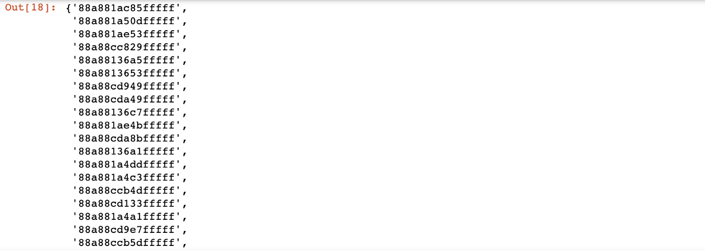
The hexs variable will return a very simple list with the IDs of all hexagons at level 8 that intersect the area provided.
Next we’ll use that list to ask the H3 API for the actual geometries that correspond to each of them. To do so, we’ll create a lambda function that passes an input (a hex ID) to the h3_to_geo_boundary method and transform the response into a shapely’s polygon.
We’ll then pass the list of IDs (the hexs variable) to the polygonise function by using python’s map method. This in turn is transformed into a list of polygons that will populate a geoseries (or a list of geopanda’s spatial types).

This is looking exactly like what we were looking for, so all that’s left is to create a geodataframe with the results and export it to a geopackage (or a shapefile if you’re old school).
This is it! We successfully extracted the h3 hexagons for our area of interest with just a few lines of code.
If you have questions or suggestions, don’t hesitate to drop me a line anytime. If you enjoyed this article, consider buying me a coffee so I keep writing more of those!
A short hands-on article on accessing Uber’s H3 hexagonal indexes using its python API

It’s now been four years since Uber open sourced its H3 grid. The company had initially developed the indexing system for ride optimization, but it turned out to be useful for all sorts of tasks that involve visualizing and exploring spatial data.
While Uber had to come up with these hexagonal hierarchichal indexes to set dynamic prices, researchers and practitioners in the geospatial field have been using grid systems to bucket events into cells for a long time. One of the most known uses of hexagons in models is Christaller’s Central Place Theory, a theory in urban geography that attempts to explain the reasons behind the distribution patterns, size, and a number of cities and towns around the world. The theory provides an hexagonal grid framework by which areas can be studied for their locational patterns.
The hexagon shape is ideal here because it allows the triangles formed by the central place vertexes to connect, and allows for each cell to touch (and potentially connect and establish a flow, for instance) with six other cells in the same way.
While hexagons suffer from less significant distortion, they cannot be perfectly subdivided nor do they align to streets. All of these limitations are addressed by the bias of clustering, aggregating cells that in turn simmulate shapes much more useful for analysis.
The H3 system provides cells with comparable shapes and sizes across the world. This provides with a potential for setting up a standard by which any spatial dataset can be set to. This means that the more spatial research use this grid, the more the datasets can be interchangeable and compared to one another.
Take for instance Montréal-based Anagraph’s demographic dataset of Canada, which used different sources — among which the Canadian 2021 population census — to model a population hexagonal grid dataset that uses the H3 index.
The same goes for influential mobility researcher Rafael Pereira, whose research on access to opportunities in Brazil makes good use of H3 indexes to better capture the spatial dynamics of phenomenons that involve movement paths or connectivity.
If you work with spatial data, you might be expecting to be able to get a link to download a shapefile somewhere. That’s not the way it’ll go here.
To get it, we’ll need to use the H3 API. In case you’re wondering, an application programming interface (API) sets the tools that can be used to make calls to (that is, to access) the server that holds the data we need. Basically this means that we can interact with this application and its data by using a set of pre-defined rules by sending certain messages to the system.
With that in mind, let’s use the methods described in the H3 API documentation to extract all polygons intersecting an area of interest. The first step will be ingesting the said area by making use of geopandas.
Now that we got ourselves a geodataframe that contains the area for which we want to extract the hexagons, let’s start using the actual H3 library. We’ll start by using h3’s polyfill method, a function that will take the geometry of the first and only feature from the geodataframe and a scale — since the H3 system is multiscalar, there are multiple sizes of hexagons we could extract — which here will be 8, the most granular level.
The hexs variable will return a very simple list with the IDs of all hexagons at level 8 that intersect the area provided.
Next we’ll use that list to ask the H3 API for the actual geometries that correspond to each of them. To do so, we’ll create a lambda function that passes an input (a hex ID) to the h3_to_geo_boundary method and transform the response into a shapely’s polygon.
We’ll then pass the list of IDs (the hexs variable) to the polygonise function by using python’s map method. This in turn is transformed into a list of polygons that will populate a geoseries (or a list of geopanda’s spatial types).
This is looking exactly like what we were looking for, so all that’s left is to create a geodataframe with the results and export it to a geopackage (or a shapefile if you’re old school).
This is it! We successfully extracted the h3 hexagons for our area of interest with just a few lines of code.
If you have questions or suggestions, don’t hesitate to drop me a line anytime. If you enjoyed this article, consider buying me a coffee so I keep writing more of those!
Denial of responsibility! Techno Blender is an automatic aggregator of the all world’s media. In each content, the hyperlink to the primary source is specified. All trademarks belong to their rightful owners, all materials to their authors. If you are the owner of the content and do not want us to publish your materials, please contact us by email – [email protected]. The content will be deleted within 24 hours.