
How to find yourself in a digital world?
The probabilistic approach to self-locate under uncertainty
Table of contents:
- What is localization and why does a robot need it?
- Why are probabilistic tools used to compute localization?
- End-to-end example: how to use bayesian algorithms to determine a robot’s position under uncertainty?
How can autonomous cars stay within a single lane at 60mph? How can an i-robot avoid falling down the stairs? How can delivery robots know if they are going to the right hungry customer? These are just a few of the questions autonomous vehicles must answer without human intervention.
1. What is localization? And why does a robot need it?
As you might imagine, accurate vehicle location is critical to whether the autonomous vehicle effectively and safely completes its tasks. The process to estimate the vehicle’s position from sensor data is called localization. Localization accuracy increases with sensors that add information and decreases with the vehicle’s movement which adds noise.
2. Why are probabilistic tools used to compute localization?
Probabilistic tools can be leveraged to improve location accuracy where neither the sensors nor the movement is 100% accurate.
What is probability?
According to the dictionary definition, probability is a “numerical description of how likely an event is to occur” (wikipedia). However, when it comes to the meaning of probability, the answer is not that simple. There are rivaling interpretations to probability from two major camps, the frequentists and bayesians.
The Frequentist approach interprets probability as the relative frequency over time; how many times will I get my desired outcome if I repeat an experiment many times?
This approach is objective because anyone who runs the experiments (e.g. flipping a coin) will get the same result in the long run.
The Bayesian approach interprets probability as the degree of certainty that an event will happen. How certain am I that I will get my desired outcome given expert knowledge and the available data? This approach is subjective, as it represents the current state of belief by combining (subjective) previous knowledge and experimental data known to date. It allows estimating the probability of a singular event that we can’t run many times, where the frequentist meaning doesn’t apply.
For example, if the probability that a date texts you back after your first meetup is 0.8, then we are 80% certain that you had a great time and the person will text you back; we don’t mean they will text 80% of the time if you repeat the first date over and over again.
What are the benefits of bayesian probability?
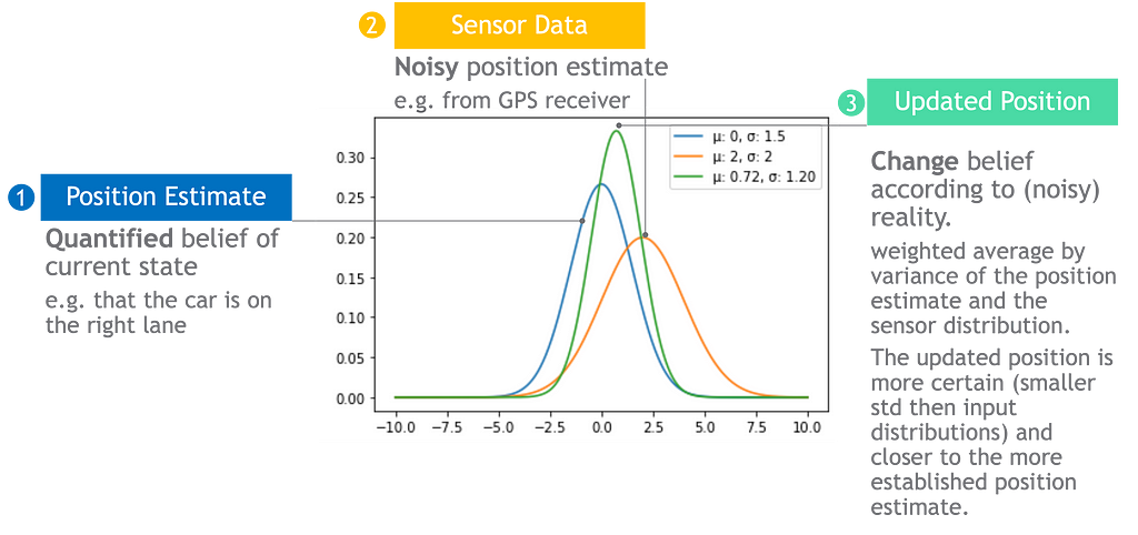
Bayesian probability allows us to both quantify our degree of belief and to update it in light of new evidence.
In our context, P(H) is our initial guess of the robot‘s position, and P(H|E) is our updated guess after measuring the sensors’ evidence E.
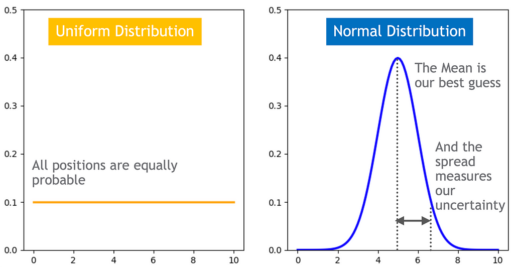
The hypothesis probability distribution quantifies our certainty in the robot’s position.
The hypothesis can change according to evidence
The more informative and accurate the sensors data, the bigger effect it will have. If the sensor is perfect, the robot’s position will align with the sensor’s reading, otherwise if the sensor data is very noisy or non-informative, the robot’s position will stay the same.
Updates can combine multiple sources of evidence
We can formulate Bayes’ law to combine multiple data sources by using the chain rule, also known as the general product rule. It permits simplifying a joint distribution of multiple evidence to a product of conditional probabilities.

For example, we often use GPS to navigate from our current location but GPS works best in clear skies and its accuracy is limited to a few meters. Autonomous cars can not solely rely on GPS to remain in a lane that is a few meters wide and to navigate in tunnels or underground parking lots. Autonomous vehicles can compensate for GPS deficiencies by adding more sources of information such as cameras.
3. End-to-end example: how to use bayesian algorithms to determine the robot’s position under uncertainty?
Let’s take a deep dive into a bayesian filter that recursively improves localization probability estimates using bayesian inference. The recursive nature means that the output of the filter at time t_0, P(H|E), serves as the hypothesis input for the next timestamp t_1, P(H).
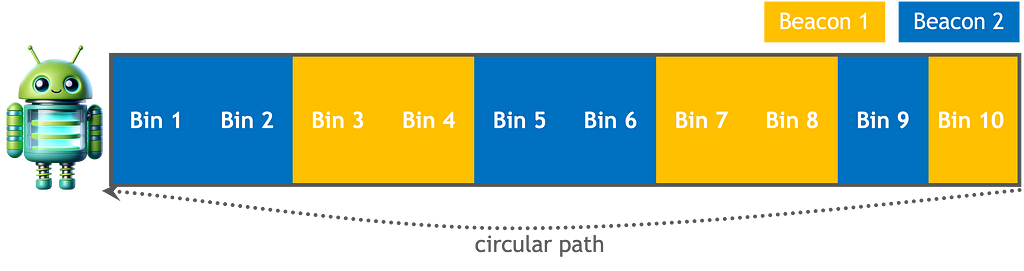
Suppose a delivery robot is looping a circular path within a space station to transport supplies. The robot has a map detailing the lay of the land and the location of sensors.
– Problem definition:
We refer to the estimated robot location as the robot’s state space. For example, a two-dimensional vector (i.e. an ordered pair of numbers) tracing x-axis position and x-axis velocity can track a robot location and changing speed in one-dimension. It is possible to extend the robot’s state space to additional dimensions to track multiple position dimensions (y, z), orientation, etc.
For simplicity, we can assume our robot is moving with constant speed. The movement adds uncertainty to the computation, since it is not 100% reliable. The engine might fail to run at a specific velocity or the robot might encounter obstacles, which will cause the robot to overshoot or undershoot its expected movement.
Our robot will sense its location by measuring the presence of a beacon. The sensor readings, also called measurement space, are not 100% accurate. Sensors might confuse noise with a beacon signal that can lead to false alarms or fail to detect a signal at all.

– The algorithm: histogram filter
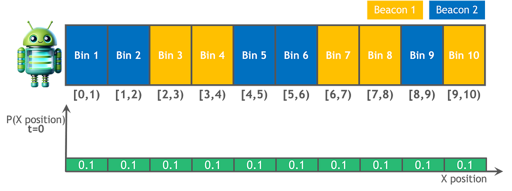
With this bayesian filter the robot state space is represented by a histogram through a finite number of bins or regions. It is a discrete filter, meaning the robot can only be in one of these regions, and we compute the probability that the robot is in each. Additionally, within each bin, such as a 5 square meter area, the probability of being at any specific point is the same. If we want to increase the granularity, we must add more bins.
This filter is non parametric, meaning it does not make any strong assumptions on the robot’s state representation, and is not restricted to one type of distribution such as a Gaussian. It is able to represent complex location estimates, such as a multimodal hypothesis that keeps multiple best guesses, but it comes with a computational cost — an exponential complexity. In order to add an additional dimension, from 1-D to 2-D while keeping the same granularity, we will need 10×10 bins, to move to 3-D we will need 10x10x10 bins, and so on. This is a significant limitation for robots that track multiple dimensions and are limited in memory and compute power.
– Calculation:
- Initial guess: We start from an unknown location equipped with a map. At the beginning every region is equally probable, as represented by a uniform distribution across all bins.
2. Movement function: simulates the robot movement. The robot’s motion is stochastic, meaning it is not guaranteed to move to the desired bin at each time step. To update the robot’s location after each move, we calculate the probability of the robot being in each region at the next time step. This calculation considers both the probability of the robot to stay in the same region and the probability of it to move to a different region.
For each movement:
  For each region:
    Region probability at time t+1 =
    Region probability at time t x stay probability +
    Probability of robot coming from the neighboring region x move probability

As shown in the equation below, the robot’s one-step movement will not change the location estimate because of the uniform distribution, where each region has equal probability to stay and move.

Even if we initially begin at a bin with complete certainty (100%), the inherent randomness in movement will gradually add noise, leading us towards a uniform distribution over time. We need to add information!
3. Sense function: incorporates measurements that add information using Bayes’ theorem.
After each movement:
    For each region:
      Region probability at time t+1 given measurement at time t+1 =
      Likelihood of the measurement given the robot is in that region
      x Region probability at time t+1 after movement
      x normlization to ensure that all the probabilities sum to 1.
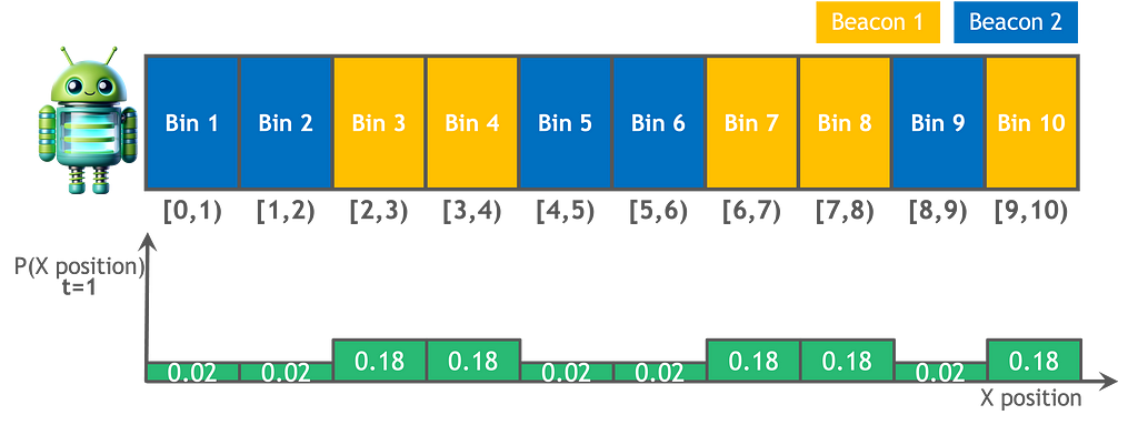
The sensors reliability is represented with probabilities, since they are not 100% accurate. The equations below demonstrate that when the sensor detects the color orange, there is a 90% probability that the robot is located in an orange bin, and a 10% probability that the sensor is wrong and the robot is actually in a blue bin.

The calculation presented below illustrates that, in contrast to movement, sensors contribute information and improve our understanding of the robot’s location. For instance, because bin 2 is not orange, the probability of the robot being in it diminishes from 0.1 to 0.02.

The image below shows the updated location hypothesis after incorporating movement and sensors’ data to our initial guess.
Final thoughts
Where is the robot? We can continuously refine our answer to this question by using recursive bayesian filters, starting from a uniform distribution that keeps all guesses equally probable until settling on the most likely one.
Bayesian filters help us measure our confidence in the robot’s whereabouts, updating this belief by integrating (noisy) sensor data with prior information (the estimated robot’s position after movement).
Sources:
- These are my summary notes from the first lectures of the highly recommend edX course “Bayesian algorithms for Self-Driving Vehicles” by Dr.Roi Yozevitch.
- Probabilistic Robotics GitBook: Non parametric filter
- Wikipedia probability, probability theory and bayes theorem
- Daniel Sabinasz’s personal blog on histogram filters
- Online converter from latex to png.
- Images: the robot avatar was created with Dall-E. All other images used in this article were created by the author.
How to find yourself in a digital world? was originally published in Towards Data Science on Medium, where people are continuing the conversation by highlighting and responding to this story.
The probabilistic approach to self-locate under uncertainty
Table of contents:
- What is localization and why does a robot need it?
- Why are probabilistic tools used to compute localization?
- End-to-end example: how to use bayesian algorithms to determine a robot’s position under uncertainty?
How can autonomous cars stay within a single lane at 60mph? How can an i-robot avoid falling down the stairs? How can delivery robots know if they are going to the right hungry customer? These are just a few of the questions autonomous vehicles must answer without human intervention.
1. What is localization? And why does a robot need it?
As you might imagine, accurate vehicle location is critical to whether the autonomous vehicle effectively and safely completes its tasks. The process to estimate the vehicle’s position from sensor data is called localization. Localization accuracy increases with sensors that add information and decreases with the vehicle’s movement which adds noise.
2. Why are probabilistic tools used to compute localization?
Probabilistic tools can be leveraged to improve location accuracy where neither the sensors nor the movement is 100% accurate.
What is probability?
According to the dictionary definition, probability is a “numerical description of how likely an event is to occur” (wikipedia). However, when it comes to the meaning of probability, the answer is not that simple. There are rivaling interpretations to probability from two major camps, the frequentists and bayesians.
The Frequentist approach interprets probability as the relative frequency over time; how many times will I get my desired outcome if I repeat an experiment many times?
This approach is objective because anyone who runs the experiments (e.g. flipping a coin) will get the same result in the long run.
The Bayesian approach interprets probability as the degree of certainty that an event will happen. How certain am I that I will get my desired outcome given expert knowledge and the available data? This approach is subjective, as it represents the current state of belief by combining (subjective) previous knowledge and experimental data known to date. It allows estimating the probability of a singular event that we can’t run many times, where the frequentist meaning doesn’t apply.
For example, if the probability that a date texts you back after your first meetup is 0.8, then we are 80% certain that you had a great time and the person will text you back; we don’t mean they will text 80% of the time if you repeat the first date over and over again.
What are the benefits of bayesian probability?
Bayesian probability allows us to both quantify our degree of belief and to update it in light of new evidence.

In our context, P(H) is our initial guess of the robot‘s position, and P(H|E) is our updated guess after measuring the sensors’ evidence E.
The hypothesis probability distribution quantifies our certainty in the robot’s position.
The hypothesis can change according to evidence
The more informative and accurate the sensors data, the bigger effect it will have. If the sensor is perfect, the robot’s position will align with the sensor’s reading, otherwise if the sensor data is very noisy or non-informative, the robot’s position will stay the same.
Updates can combine multiple sources of evidence
We can formulate Bayes’ law to combine multiple data sources by using the chain rule, also known as the general product rule. It permits simplifying a joint distribution of multiple evidence to a product of conditional probabilities.
For example, we often use GPS to navigate from our current location but GPS works best in clear skies and its accuracy is limited to a few meters. Autonomous cars can not solely rely on GPS to remain in a lane that is a few meters wide and to navigate in tunnels or underground parking lots. Autonomous vehicles can compensate for GPS deficiencies by adding more sources of information such as cameras.
3. End-to-end example: how to use bayesian algorithms to determine the robot’s position under uncertainty?
Let’s take a deep dive into a bayesian filter that recursively improves localization probability estimates using bayesian inference. The recursive nature means that the output of the filter at time t_0, P(H|E), serves as the hypothesis input for the next timestamp t_1, P(H).
Suppose a delivery robot is looping a circular path within a space station to transport supplies. The robot has a map detailing the lay of the land and the location of sensors.
– Problem definition:
We refer to the estimated robot location as the robot’s state space. For example, a two-dimensional vector (i.e. an ordered pair of numbers) tracing x-axis position and x-axis velocity can track a robot location and changing speed in one-dimension. It is possible to extend the robot’s state space to additional dimensions to track multiple position dimensions (y, z), orientation, etc.
For simplicity, we can assume our robot is moving with constant speed. The movement adds uncertainty to the computation, since it is not 100% reliable. The engine might fail to run at a specific velocity or the robot might encounter obstacles, which will cause the robot to overshoot or undershoot its expected movement.
Our robot will sense its location by measuring the presence of a beacon. The sensor readings, also called measurement space, are not 100% accurate. Sensors might confuse noise with a beacon signal that can lead to false alarms or fail to detect a signal at all.
– The algorithm: histogram filter
With this bayesian filter the robot state space is represented by a histogram through a finite number of bins or regions. It is a discrete filter, meaning the robot can only be in one of these regions, and we compute the probability that the robot is in each. Additionally, within each bin, such as a 5 square meter area, the probability of being at any specific point is the same. If we want to increase the granularity, we must add more bins.
This filter is non parametric, meaning it does not make any strong assumptions on the robot’s state representation, and is not restricted to one type of distribution such as a Gaussian. It is able to represent complex location estimates, such as a multimodal hypothesis that keeps multiple best guesses, but it comes with a computational cost — an exponential complexity. In order to add an additional dimension, from 1-D to 2-D while keeping the same granularity, we will need 10×10 bins, to move to 3-D we will need 10x10x10 bins, and so on. This is a significant limitation for robots that track multiple dimensions and are limited in memory and compute power.
– Calculation:
- Initial guess: We start from an unknown location equipped with a map. At the beginning every region is equally probable, as represented by a uniform distribution across all bins.
2. Movement function: simulates the robot movement. The robot’s motion is stochastic, meaning it is not guaranteed to move to the desired bin at each time step. To update the robot’s location after each move, we calculate the probability of the robot being in each region at the next time step. This calculation considers both the probability of the robot to stay in the same region and the probability of it to move to a different region.
For each movement:
  For each region:
    Region probability at time t+1 =
    Region probability at time t x stay probability +
    Probability of robot coming from the neighboring region x move probability
As shown in the equation below, the robot’s one-step movement will not change the location estimate because of the uniform distribution, where each region has equal probability to stay and move.
Even if we initially begin at a bin with complete certainty (100%), the inherent randomness in movement will gradually add noise, leading us towards a uniform distribution over time. We need to add information!
3. Sense function: incorporates measurements that add information using Bayes’ theorem.
After each movement:
    For each region:
      Region probability at time t+1 given measurement at time t+1 =
      Likelihood of the measurement given the robot is in that region
      x Region probability at time t+1 after movement
      x normlization to ensure that all the probabilities sum to 1.
The sensors reliability is represented with probabilities, since they are not 100% accurate. The equations below demonstrate that when the sensor detects the color orange, there is a 90% probability that the robot is located in an orange bin, and a 10% probability that the sensor is wrong and the robot is actually in a blue bin.
The calculation presented below illustrates that, in contrast to movement, sensors contribute information and improve our understanding of the robot’s location. For instance, because bin 2 is not orange, the probability of the robot being in it diminishes from 0.1 to 0.02.
The image below shows the updated location hypothesis after incorporating movement and sensors’ data to our initial guess.
Final thoughts
Where is the robot? We can continuously refine our answer to this question by using recursive bayesian filters, starting from a uniform distribution that keeps all guesses equally probable until settling on the most likely one.
Bayesian filters help us measure our confidence in the robot’s whereabouts, updating this belief by integrating (noisy) sensor data with prior information (the estimated robot’s position after movement).
Sources:
- These are my summary notes from the first lectures of the highly recommend edX course “Bayesian algorithms for Self-Driving Vehicles” by Dr.Roi Yozevitch.
- Probabilistic Robotics GitBook: Non parametric filter
- Wikipedia probability, probability theory and bayes theorem
- Daniel Sabinasz’s personal blog on histogram filters
- Online converter from latex to png.
- Images: the robot avatar was created with Dall-E. All other images used in this article were created by the author.
How to find yourself in a digital world? was originally published in Towards Data Science on Medium, where people are continuing the conversation by highlighting and responding to this story.
Denial of responsibility! Techno Blender is an automatic aggregator of the all world’s media. In each content, the hyperlink to the primary source is specified. All trademarks belong to their rightful owners, all materials to their authors. If you are the owner of the content and do not want us to publish your materials, please contact us by email – [email protected]. The content will be deleted within 24 hours.