How to Learn Causal Inference on Your Own for Free

By Jessie Hobb On Feb 21, 2024

The ultimate self-study guide for all levels

Image by author

While everyone focuses on AI and predictive inference, standing out requires mastering not just prediction, but understanding the “why” behind the data — in other words, mastering causal inference.

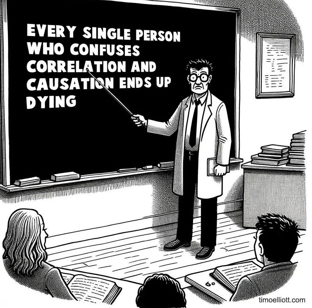
You have heard that “correlation does not imply causation”, but few truly grasp its implications or know when to confidently assert causality.

The distinction between predictive inference and causal inference is profound, with the latter often overlooked, leading to costly mistakes. The logic and models between the two approaches are vastly different and this guide aims to equip you with the knowledge to discern causal relationships with confidence.

Results from Google Trends for “causal inference” revealing the recent quickly growing interest and the association with machine learning. Image by author

I am convinced that causal inference is arguably one of the most valuable skills to acquire today for three reasons:

It is tremendously useful for virtually any job, extending beyond data scientists to include business leaders and managers (see next Section).
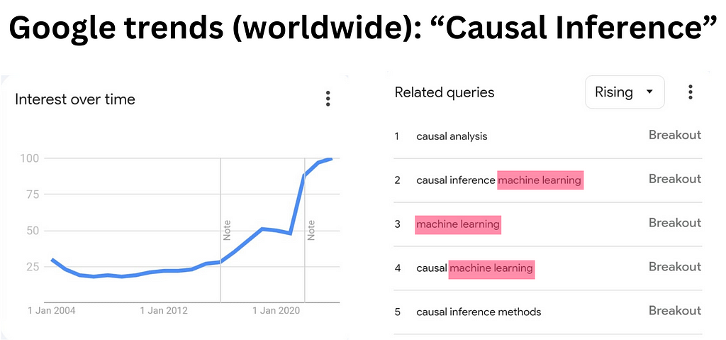
It remains a niche and few people are experts in this field and the interest is growing fast (cf. image above).
As revealed by the Google Trends results (see image above), “causal machine learning” is the latest associated trend. Hence, knowing causal inference will help you connect this knowledge with the current AI focus and put you one step ahead.

To help you master causal inference and have a valuable asset on the job market and beyond, I crafted this self-study guide, suitable for all levels, requiring no prerequisites, and composed exclusively of free online resources.

Plan of the guide:

Introduction: Causal inference key concepts
Technical tools
Randomized Experiments (A/B testing)
Quasi-experimental design
Advanced topics
Conclusion

https://medium.com/media/32458105d191e4ac0d12aeb11883482d/href

1. Introduction: Causal inference key concepts

Causality, the field focused on understanding the relationships between cause and effect, seeks to answer critical questions such as ‘Why?’ and ‘What if?’. Understanding the concept of causality is crucial from fighting climate change, to our quest for happiness, including strategic decisions making.

Examples of major questions requiring causal inference:

What impact might banning fuel cars have on pollution?
What are the causes behind the spread of certain health issues?
Could reducing screen time lead to increased happiness?
What is the Return On Investment of our ad campaign?

In what follows I will essentially refer to two free e-books available with Python code and data to play with. The first e-book offers quick overviews, while the second allows for a more in-depth exploration of the content.

Causal Inference for the Brave and True by Matheus Facure

2. Causal Inference: The Mixtape by Scott Cuningham

1.1 The fundamental problem of causal inference

Let’s dive into the most fundamental concept necessary to understand causal inference through a situation we might all be familiar with.

Imagine that you have been working on your computer all day long, a deadline is approaching, and you start to feel a headache coming on. You still have a few hours of work ahead, so you decide to take a pill. After a while, your headache is gone.

But then, you start questioning: Was it really the pill that made the difference? Or was it because you drank tea or took a break? The fascinating but eventually also frustrating part is that it is impossible to answer this question as all those effects are confounded.

The only way to know for certain if it was the pill that cured your headache would be to have two parallel worlds.

In one of the two worlds you take the pill, and in the other, you don’t, or you take a placebo ideally. You can only prove the pill’s causal effect if you feel better in the world where you took the pill, as the pill is the only difference between the two worlds.

Unfortunately, we do not have access to parallel worlds to experiment with and assess causality. Hence, many factors occur simultaneously and are confounded (e.g., taking a pill for a headache, drinking tea, and taking a break; increasing ad spending during peak sales seasons; assigning more police officers to areas with higher crime rates, etc.).

To quickly grasp this fundamental concept in more depth without requiring any additional technical knowledge, you can dive into the following article on Towards Data Science:

📚 Resource:

The Science and Art of Causality (part 1)

1.2 A little bit of formalization: Potential Outcomes

Now that you understand the basic idea, it is time to go further and theoretically formalize these concepts. The most common approach is the potential outcomes framework, which allows for the clear articulation of model assumptions. These are essential for specifying the problems and identifying the solutions.

The central notation used in this model are:

Yᵢ(0) represents the potential outcome of individual i without the treatment.
Yᵢ(1) represents the potential outcome of individual i with the treatment.

Note that various notations are used. The reference to the treatment (1 or 0) may appear in parentheses (as used above), in superscript, or subscript. The letter “Y” refers to the outcome of interest, such as a binary variable that takes the value one if a headache is present and zero otherwise. The subscript “i” refers to the observed entity (e.g., a person, a lab rat, a city, etc.). Finally, the term ‘treatment’ refers to the ‘cause’ you are interested in (e.g., a pill, an advertisement, a policy, etc.).

Using this notation, we can refer to the fundamental problem of causal inference by stating that it is impossible to observe both Yᵢ(0) and Yᵢ(1) simultaneously. In other words, you never observe the outcome for the same individual with and without the treatment at the same time.

While we cannot identify the individual effect Yᵢ(1)-Yᵢ(0), we can measure the Average Treatment Effect (ATE): E[Yᵢ(1)-Yᵢ(0)]. However, this Average Treatment Effect is biased if you have systematic differences between the two groups other than the treatment.

To go beyond this short introduction you can refer to the two following chapters:

📚Resources:

Brief overview: The potential outcomes (Causal Inference for the brave and true)
In-depth: The potential outcomes (Causal Inference: The Mixtape)

1.3 Visual representation of causal links: Directed (Acyclic) Graphs

Visual representations are powerful tools for reducing mental load, clarifying assumptions, and facilitating communication. In causal inference, we use directed graphs. As the name suggests, these graphs depict various elements (e.g., headache, pill, tea) as nodes, connected by unidirectional arrows that illustrate the direction of causal relationships. (Note: I deliberately omit mentioning the common assumption of ‘Acyclicity’ associated with these graphs, as it goes beyond the scope of this overview but is discussed in the second reference available at the end of this subsection.)

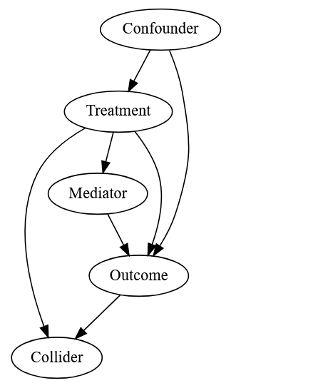
Example of a Directed Graph, image by author

Causal inference primarly differs from predictive inference due to the assumed underlying causal relationships. Those relationships are explicitly represented using this special kind of graph called Directed (Acyclic) Graphs. This tool jointly with the potential outcome framework is at the core of causal inference and will allow thinking clearly about the potential problems and, consequently, solutions for assessing causality

📚Resources:

Short intro: Directed Acyclic Graph (Causal Inference for the brave and true)
In-depth: Directed Acyclic Graph (Causal Inference: The Mixtape)

2. Technical Tools

If you want to go further and apply these methods to data, you will need to be equipped with two technical tools

A foundational understanding of probability, statistics, and linear regression.
Knowledge of a statistical software

2.1 Probability, Statistics, and Linear regression

These tools are valuable for data science in general, and you can concentrate specifically on what matters most. Furthermore, there is a chapter dedicated to this topic in both of the reference books including exclusively on the concepts useful for causal inference:

📚Resources:

In addition, in my opinion, one of the most valuable yet often disregarded topics related to linear regression is the concept of “bad controls”. Understanding what you should control for and what will actually create problems is key. The following two references will allow you to grasp this concept.

📚Resources:

Finally, understanding Fixed Effects regression is essential for causal inference. This type of regression allows us to account for numerous confounding factors that might be impossible to measure (e.g., culture) or for which data is simply unavailable.

📚Resources:

Short intro: Fixed Effects (Causal Inference for the brave and true)
In depth: Fixed Effects (Causal Inference: The Mixtape)

2.2 Statistical tool

Numerous tools allow us to do causal inference and statistical analysis, and in my opinion, the best among them are STATA, Python, and R.

STATA is specifically designed for statistics, particularly econometrics, making it an incredibly powerful tool. It offers the latest packages from cutting-edge research. However, it is expensive and not versatile.

Python, on the other hand, is the leading programming language today. It is open-source and highly versatile, which are key reasons why it’s my preferred choice. Additionally, ChatGPT performs very well with Python-related queries which is an important advantage in this AI era.

R is very powerful for statistics. The debate between R and Python is ongoing, and I leave the judgment to you. Note that R is less versatile than Python, and it appears that ChatGPT’s proficiency with R is not as strong. Additionally, the two main books I reference contain Python code (‘Causal Inference for the Brave and True’; ‘Causal Inference: The Mixtape’). This further supports focusing on Python.

There are millions of free resources to learn Python from scratch (please comment if you have better suggestions). But here are the ones I would typically recommend if you start from zero (you never coded):

📚Resources:

3. Randomized Experiments (A/B testing)

In the first section of this guide, we discovered the fundamental problem of causal inference. This problem highlighted the difficulty of assessing causality. So what can we do?

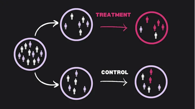
Usually, the first solution presented and considered the “gold standard” in causal inference, is randomized experiments (Randomized Controlled Trials).

Essentially, the idea behind randomized experiments is to replicate, or at least approach as much as possible, a parallel world scenario. This allows us to isolate the effect (the consequence) of the treatment (the cause).

As explained in my Towards Data Science article mentioned in Section 1:

“We take a sample that is, hopefully, representative of a larger population, and randomly allocate subjects between two groups (treatment and control) or more. The subjects typically do not know whether they receive the treatment or not (a process known as blinding). Therefore, the two groups are arguably comparable. Since the only difference is the treatment, if we observe an effect, it is potentially causal, provided that no other biases exist.”

Simple representation of a Randomized Experiment. Image by author

📚Resource:

4. Quasi-experimental design

Controlled experiments are not always possible (e.g. changing the sex/origin for studying discrimination) or ethical (e.g. exposing humans to lethal doses of pollutant to study respiratory disease).

Moreover, Randomized experiments tend to have a very strong internal validity but a weaker external validity. Internal validity means that it allows within the scope of the study to measure precisely causality, while external validity refers to the capacity to extrapolate the results beyond the scope of the study.

One of the main limitation of controlled experiments is the external validity. Image by author.

For example, medical research relies extensively on inbred strains of rats/mice. Those animals have almost an identical genetic code, they live the same lab life, eat the same food, etc. Hence, when you do a controlled experiment with such animals you are very close to the parallel world situation working almost with clones. However, the external validity is weaker due to the homogeneity of the study subjects. Moreover, often in controlled experiments the whole environment is controlled and in some cases, it makes the situation a bit unrealistic and reduces the usefulness of the results.

Let me illustrate this point with the following research paper. A study published in the British Medical Journal (one of the most prestigious medical journals), found no effect of using a parachute when jumping from an airplane on the “Composite of death or major traumatic injury” (Yeh et al. (2018)). In this randomized experiment, the participants jumped from a small, stationary airplane on the ground. This absurd setup illustrates the issue that often arises in controlled experiments when the setup is unrealistic. The purpose of the paper is to raise awareness in medical research about the issue of external validity, which is a current and serious concern.

One way to address this issue is by relying on other methods, known as quasi-experimental designs. The idea is to observe a quasi-random allocation between groups in natural settings. ‘Quasi-random’ means that the allocation is effectively as good as random once we isolate or control for potential systematic differences.

4.1 Example

To illustrate the concept of quasi-experimental design, I will explain the intuition behind one of the methods called Regression Discontinuity Design (RDD) used to measure the impact of alcohol consumption on mortality.

The idea behind a RDD is to exploit a discontinuity in treatment allocation (e.g., a geographical border, an age-related administrative law, etc.) where individuals or places very similar to each other receive different treatments based on a cutoff point.

For instance, in the study “The Effect of Alcohol Consumption on Mortality” by Carpenter and Dobkin (2009), the authors used the discontinuity at the minimum legal drinking age to examine the immediate effect of alcohol consumption on mortality.

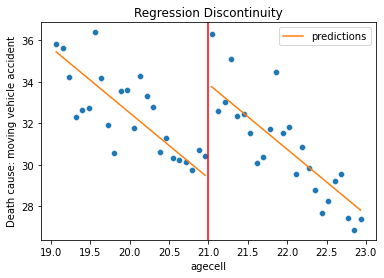
The mortality rate related to moving vehicle accidents jumps suddenly when people turn 21 years old arguably caused by alcohol consumption. Replication of (Carpenter and Dobkin (2009)) main result. Image by author.

The rationale in this study is that individuals who consume alcohol are not usually comparable to those who don’t due to many other systematic differences (e.g. age, socio-economic statuts, risk of various diseases, etc.). However, by comparing individuals just below and just above the age of 21, one can argue they are very similar, assuming no other significant changes occur at that age. This approach allows for a clearer attribution of changes in mortality rates to alcohol consumption. This example, complete with data and code, is also included in the first reference provided at the end of the next sub-section 4.2 Methods.

4.2 Methods

There are numerous methods available. However, I recommend you learn the following three methods in this order:

Regression Discontinuity Design (RDD)
Difference-in-Differences (Diff-in-Diff)
Instrumental Variables (IV)

These three methods are standard in academic research but are also used in the industry. Together, they will provide a toolbox that allows you to address causal questions in various settings.

📚Resources:

Short intro: Regression Discontinuity Design (Causal Inference for the brave and true)
In depth: Regression Discontinuity Design (Causal Inference: The Mixtape)
Short intro: Diff-in-Diff (Causal Inference for the brave and true)
In depth: Diff-in-Diff (Causal Inference: The Mixtape)
Example of Diff-in-Diff: ChatGPT effect on Stack Overflow
Short intro: Instrumental Variables (Causal Inference for the brave and true)
In depth: Instrumental Variables (Causal Inference: The Mixtape)

6. Advanced topics

Of course, causal inference is very rich. Mastering those tools will already equip you very well to work in causal inference. However, other potential topics could be explored as well. Here is a list:

📚 Synthetic Control (very popular and fastest growing quasi-experimental method) :

Short intro: Synthetic Control (Causal Inference for the brave and true)
Short intro: Synthetic Diff-in-Diff (Causal Inference for the brave and true)
In depth: Synthetic Control (Causal Inference: The Mixtape)

📚 Causal Machine Learning (joining the best of the two worlds of causal inference and Machine Learning):

Machine Learning & Causal Inference: A Short Course (Stanford University)
Causal Machine Learning: A Survey and Open Problems ((Kaddour et al. 2022))
!Not Free! Causal Analysis: Impact Evaluation and Causal Machine Learning with Applications in R (Martin Huber)

📚 Causal Discovery

!Not Free! Causal Inference and Discovery in Python

6. Conclusion

Following this guide will equip you with a solid theoretical foundation and a comprehensive toolbox for incorporating causal inference into your skillset. These concepts extend beyond measuring causal effects for your job; they enhance your critical thinking abilities. Abusive causal claims are widespread in the news, politics, by ‘experts’, managers, and others. Applying these concepts can reduce the risk of manipulation. This toolbox can also be valuable in everyday discussions with friends or during team meetings when making decisions or reflecting on observations.

Of course, this is just the beginning. To fully integrate and master these skills, practice is essential. I encourage you to select a relevant question, find data, and use the tools provided in this guide to attempt to answer it. Then, include this project in your portfolio to showcase your new knowledge.

Enjoy this exciting journey on the path to answerig the never-ending question of ‘Why?’.

How to Learn Causal Inference on Your Own for Free was originally published in Towards Data Science on Medium, where people are continuing the conversation by highlighting and responding to this story.

The ultimate self-study guide for all levels

You have heard that “correlation does not imply causation”, but few truly grasp its implications or know when to confidently assert causality.

I am convinced that causal inference is arguably one of the most valuable skills to acquire today for three reasons:

It is tremendously useful for virtually any job, extending beyond data scientists to include business leaders and managers (see next Section).
It remains a niche and few people are experts in this field and the interest is growing fast (cf. image above).
As revealed by the Google Trends results (see image above), “causal machine learning” is the latest associated trend. Hence, knowing causal inference will help you connect this knowledge with the current AI focus and put you one step ahead.

To help you master causal inference and have a valuable asset on the job market and beyond, I crafted this self-study guide, suitable for all levels, requiring no prerequisites, and composed exclusively of free online resources.

Plan of the guide:

Introduction: Causal inference key concepts
Technical tools
Randomized Experiments (A/B testing)
Quasi-experimental design
Advanced topics
Conclusion

https://medium.com/media/32458105d191e4ac0d12aeb11883482d/href

1. Introduction: Causal inference key concepts

Examples of major questions requiring causal inference:

What impact might banning fuel cars have on pollution?
What are the causes behind the spread of certain health issues?
Could reducing screen time lead to increased happiness?
What is the Return On Investment of our ad campaign?

Causal Inference for the Brave and True by Matheus Facure

2. Causal Inference: The Mixtape by Scott Cuningham

1.1 The fundamental problem of causal inference

Let’s dive into the most fundamental concept necessary to understand causal inference through a situation we might all be familiar with.

The only way to know for certain if it was the pill that cured your headache would be to have two parallel worlds.

To quickly grasp this fundamental concept in more depth without requiring any additional technical knowledge, you can dive into the following article on Towards Data Science:

📚 Resource:

The Science and Art of Causality (part 1)

1.2 A little bit of formalization: Potential Outcomes

The central notation used in this model are:

Yᵢ(0) represents the potential outcome of individual i without the treatment.
Yᵢ(1) represents the potential outcome of individual i with the treatment.

To go beyond this short introduction you can refer to the two following chapters:

📚Resources:

Brief overview: The potential outcomes (Causal Inference for the brave and true)
In-depth: The potential outcomes (Causal Inference: The Mixtape)

1.3 Visual representation of causal links: Directed (Acyclic) Graphs

📚Resources:

Short intro: Directed Acyclic Graph (Causal Inference for the brave and true)
In-depth: Directed Acyclic Graph (Causal Inference: The Mixtape)

2. Technical Tools

If you want to go further and apply these methods to data, you will need to be equipped with two technical tools

A foundational understanding of probability, statistics, and linear regression.
Knowledge of a statistical software

2.1 Probability, Statistics, and Linear regression

📚Resources:

Short intro: Fixed Effects (Causal Inference for the brave and true)
In depth: Fixed Effects (Causal Inference: The Mixtape)

2.2 Statistical tool

Numerous tools allow us to do causal inference and statistical analysis, and in my opinion, the best among them are STATA, Python, and R.

📚Resources:

3. Randomized Experiments (A/B testing)

In the first section of this guide, we discovered the fundamental problem of causal inference. This problem highlighted the difficulty of assessing causality. So what can we do?

Usually, the first solution presented and considered the “gold standard” in causal inference, is randomized experiments (Randomized Controlled Trials).

As explained in my Towards Data Science article mentioned in Section 1:

“We take a sample that is, hopefully, representative of a larger population, and randomly allocate subjects between two groups (treatment and control) or more. The subjects typically do not know whether they receive the treatment or not (a process known as blinding). Therefore, the two groups are arguably comparable. Since the only difference is the treatment, if we observe an effect, it is potentially causal, provided that no other biases exist.”

📚Resource:

4. Quasi-experimental design

Controlled experiments are not always possible (e.g. changing the sex/origin for studying discrimination) or ethical (e.g. exposing humans to lethal doses of pollutant to study respiratory disease).

4.1 Example

4.2 Methods

There are numerous methods available. However, I recommend you learn the following three methods in this order:

Regression Discontinuity Design (RDD)
Difference-in-Differences (Diff-in-Diff)
Instrumental Variables (IV)

These three methods are standard in academic research but are also used in the industry. Together, they will provide a toolbox that allows you to address causal questions in various settings.

📚Resources:

Short intro: Regression Discontinuity Design (Causal Inference for the brave and true)
In depth: Regression Discontinuity Design (Causal Inference: The Mixtape)
Short intro: Diff-in-Diff (Causal Inference for the brave and true)
In depth: Diff-in-Diff (Causal Inference: The Mixtape)
Example of Diff-in-Diff: ChatGPT effect on Stack Overflow
Short intro: Instrumental Variables (Causal Inference for the brave and true)
In depth: Instrumental Variables (Causal Inference: The Mixtape)

6. Advanced topics

📚 Synthetic Control (very popular and fastest growing quasi-experimental method) :

Short intro: Synthetic Control (Causal Inference for the brave and true)
Short intro: Synthetic Diff-in-Diff (Causal Inference for the brave and true)
In depth: Synthetic Control (Causal Inference: The Mixtape)

📚 Causal Machine Learning (joining the best of the two worlds of causal inference and Machine Learning):

Machine Learning & Causal Inference: A Short Course (Stanford University)
Causal Machine Learning: A Survey and Open Problems ((Kaddour et al. 2022))
!Not Free! Causal Analysis: Impact Evaluation and Causal Machine Learning with Applications in R (Martin Huber)

📚 Causal Discovery

!Not Free! Causal Inference and Discovery in Python

6. Conclusion

Enjoy this exciting journey on the path to answerig the never-ending question of ‘Why?’.

Read original article here

Denial of responsibility! Techno Blender is an automatic aggregator of the all world’s media. In each content, the hyperlink to the primary source is specified. All trademarks belong to their rightful owners, all materials to their authors. If you are the owner of the content and do not want us to publish your materials, please contact us by email – [email protected]. The content will be deleted within 24 hours.