
Image generation with diffusion models using Keras and TensorFlow
Using Diffusion to generate images
You must have heard of Dall-E 2. Published by Open AI, which is a model that generates realistic looking images from a given text prompt. You can check out a smaller version of the model here.
Ever wondered how it works under the hood? Well… it uses a new class of generative technique, called ‘diffusion’. The idea was proposed by Sohl-Dickstein, et al in 2015, where essentially, a model generates an image from Noise.
But why use diffusion models when there are GANs around?
GANs are great at generating high fidelity images. But, as outlined in this paper by Open AI: Diffusion models beat GANs on Image Synthesis, diffusion models are much better at image synthesis by being more faithful to the image. GANs have to produce an image in one go and generally don’t have any options for refinement during the generation of the image. Diffusion on the other hand is a slow and iterative process, during which, noise is converted into image, step by step. This allows diffusion models to have better options for guiding the image towards the desired result.
In this article we will be looking at how to create our own diffusion model based on Denoising Diffusion Probabilistic Models (Ho et al, 2021)(DDPM) and Denoising Diffusion Implicit Models (Song et al, 2021)(DDIM) using Keras and TensorFlow. So lets get started…
The process behind diffusion models is divided into two parts:
– Forward Noising process, and
– Backward Denoising process.
Forward Noising:
The concept of diffusion models is based on the well researched concept of diffusion in Physics.
In Physics, diffusion is defined as a process in which an isolated system tries to attain homogeneity by by altering the potential gradient in response to the introduction of a new element.
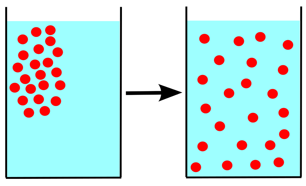
Using diffusion models, we try to reverse this process of homogenization by predicting the movements of the new element one step at a time.
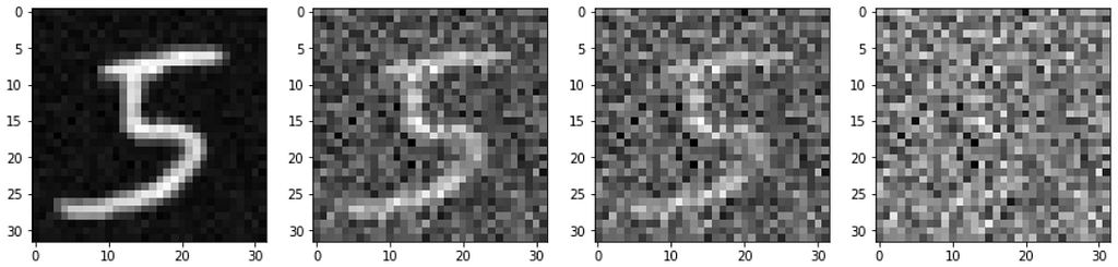
Consider the series of images given below. Here we see that we gradually add small amounts of random noise to the image till it becomes indistinguishable. Our diffusion model, will try to figure out how to reverse this process of adding noise.
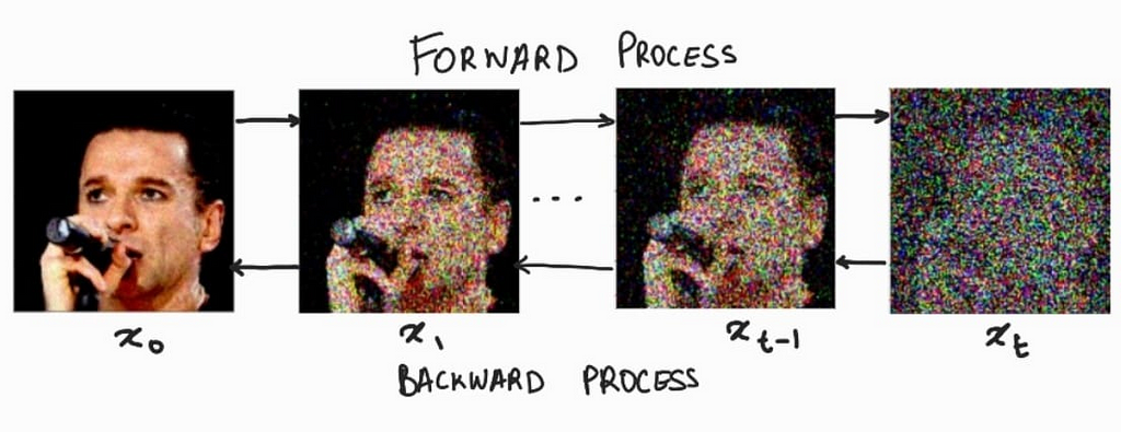
For the forward noising process q, we define a Markov Chain for a predefined amounts of steps, say T. Which takes an image and adds small amounts of Gaussian Noise to the image according to a variance schedule: β₀, β₁, … βt. Where β₀ < β₁< … < βt.
We then train a model that learns to remove this small amounts of noise at every timestep(given that the added noise is in small increments). We will explore this in the backward denoising section.
But first, what is a Markov Chain??
A Markov chain is a chain of events in which an event is only determined by the previous event.
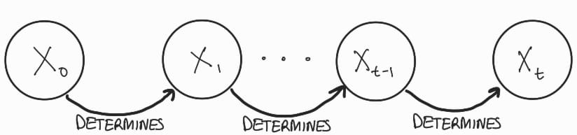
Here, the state x1 is only determined by using x0, x2 by x1, and so on till we reach xT. So for our purpose, x0 state is our normal image, and as we move forward on our Markov chain, the image gets noisier till we reach the state xT.
Addition of Noise:
According to our Markov chain, the state xt is only determined by the state xt-1. For this, we need to calculate the probability q(xt|xt-1) to generate a slightly noisier image at the time-step t compared to t-1. This ‘slightly’ noisier image is generated by sampling small amount of noise using the Gaussian Distribution ‘N’ and adding it to the image. Noise sampled from Gaussian distribution is only determined by the mean and standard deviation. Here’s where we use the variance schedule: β₀, β₁, … βt. We make the mean value depended on βt and the input image xt. So finally, q(xt|xt-1) can be defined as:

And according to principle of Markov chains, the probability that a chain from x1 to xT occurs, for a given initial state x0 is given by:

Reparameterization:
The role of our model is to undo the added noise at every timestamp. To generate the noisy image at the said timestamp, we need to iterate through the Markov chain till we obtain the desired noisy image. This process is very inefficient. As a work around, we use a reparameterization trick, which uses an approximation to generate the noise at the required timestamp. This trick works because the sum of two gaussian samples is also a gaussian sample. Here’s the reparameterization formula:
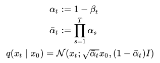
Therefore, we can pre-calculate the values for α and α bar, using the formula for q(xt|x0), obtain the noised image xt at the timestep t given the original image x0.
Enough theory, lets code this…
Here are the dependencies that we will need in order to build our model.
!pip install tensorflow
!pip install tensorflow_datasets
!pip install tensorflow_addons
!pip install einops
Lets start with the imports
https://medium.com/media/85519f6dc407476c423f001aed9375f9/href
For this implementation, we will use the MNIST digits dataset.
https://medium.com/media/16b8393afc207288c92a8cb3c350888e/href
As per the description of the forward diffusion process, we need to create a fixed beta schedule. Along with that let us also setup the forward noising process and timestamp generation.
https://medium.com/media/ad7ed03bf93804575d961c55be0c247e/href
now lets visualize the forward noising process.
https://medium.com/media/51e2f43218afbf75ff8329df13b866cc/href
Backward Denoising:
Lets understand what exactly will our model do..
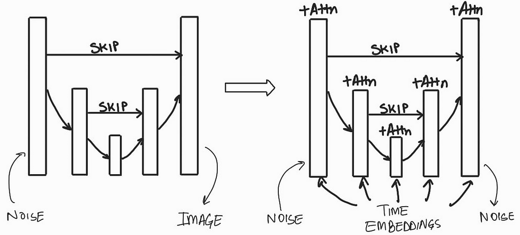
We want a image generating model that will predict what noise was added to the image at a given timestamp. This model should take in an input of noised image along with the timestamp and predicts what noise was added to the image at that time step. A U-Net style model is perfect for this job. We can make some changes to the base architecture by changing the Convolutional layers to ResNet layers, add mechanisms to consider timestamp encodings, and also have attention layers. The U-Net model was first proposed for biomedical image segmentation but since its inception, it has been modified and used for a lot of different applications.
Let code up our U-Net
1) Helper modules
https://medium.com/media/61d7c5db6adbe888e631691157cb4225/href
2) Building blocks of the U-Net model:
Here we are incorporating time embedding by scaling and shifting the input passed to the resnet block. This scale and shift factor comes by passing the time embeddings through a Multi Layer Perceptron(MLP) module within the resnet block. This MLP will convert the fixed sized time embeddings into a vector that is complient with the compatible dimensions of the blocks in the resnet layer. Scale and Shift is written as ‘Gamma’ and ‘Beta’ in the code below.
https://medium.com/media/1a0175db381fa050cb0eb69f2224a006/href
3) U-Net model
https://medium.com/media/b8eb49479e6b6e8b5b927590b3a960ce/href
Once, we have defined our U-Net model, we can now create an instance of it along with a checkpoint manager to save checkpoints during training. While we are at it, lets also create our optimizer. We will use the Adam optimizer with a learning rate of 1e-4.
https://medium.com/media/2e8493b1cb996f342d451d70ff6e03df/href
Training our model:
The backward denoising step for our model is define by p, where p is:

Here we want our model, i.e., our U-Net model, to predict the noise in the input image xt at a given timestep t by essentially predicting the value of µ(xt, t) and Σ(xt, t), i.e., the mean and variance for xt at the timestep t. We calculate the loss for the predicted noise between the predicted noise Є_θ and the original noise Є by the following formula:

The formula may look intimidating to few folks, but we are going to be essentially calculating the loss value using Mean Squared Error between the predicted noise and the real noise. So lets code this up!
https://medium.com/media/a6b9461610230a2c090aec5f95c2a5bc/href
For the training process, we will use the following algorithm:
1) Generate a random number for the generation of timestamps and noise.
2) Create a list of random timestamps according to the batch size
3) Run the input image through the forward noising process along with the timestamps.
4) Get the predictions from the U-Net model using the noised image and the timestamps.
5) Calculate the loss between the predicted noise and real noise.
6) Update the trainable variables in the U-Net model.
7) Repeat for all training batches.
https://medium.com/media/276edfc55271e506fceabd1813f54fe0/href
Now that our model is trained, lets run it in inference mode. In the DDPM paper, the authors had outlined an algorithm for inference.
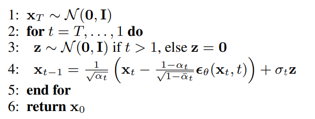
Here xt is a random sample, which we pass through our U-Net model and obtain Є_θ, then we calculate xt-1according to the formula:

Before we code this, lets create a helper function that will create and save a gif file from a list of images.
https://medium.com/media/7acc855b45990c882f6404e11773fb6a/href
Now lets make our backward denoising algorithm using the DDPM approach.
https://medium.com/media/868c1f80593dfe571e6fe7c991f4f3d1/href
now for the inference, lets create a random image using the function defined above.
https://medium.com/media/7f6adae6aeda0520cb843e4f0545368e/href
Here’s an example GIF generated by using the DDPM inference algorithm:
There’s one problem with the inference algorithm proposed in the DDPM paper. The process is very slow since we have to loop through all 200 timesteps to get the result. To make this process faster, an improved inference loop was proposed in the DDIM paper. Lets discuss that..
DDIM:
In the DDIM paper, the authors proposed a non-markovian method for backward denoising process, therefore removing the constraint that the order of the chain has to depend on the previous image. The paper proposed a modification to the DDPM objective by making the loss function more general:

From this loss function, we can infer that the loss value is only dependent on q(xt|x0) and not the join probability of q(x1:T|x0). Along with this, the authors also proposed that we can explore a different inference approach which is non-markovian. Complicated looking math coming up:
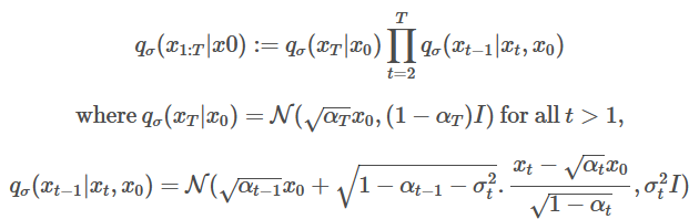
The above changes make the forward process non-Markovian as well where σ controls the stochasticity of the forward process. When σ→0, we reach a case where xt−1 becomes known and fixed. For the generative process with a fixed prior pθ(xT)=N(0,I):

Finally the formula for inference is given by:
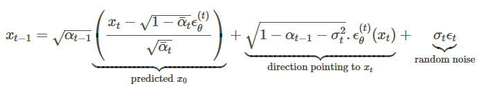
Here, if we set σ=0 ∀ t then the forward process becomes deterministic.
Above formulae are taken from [1].
Enough mathematics, lets code this up.
https://medium.com/media/1093a3225718d0b7c37b934fbdd6846e/href
Now lets use a similar backward denoising process as DDPM. Note that we are using only 10 steps for this inference loop, instead of the 200 steps of DDPM
https://medium.com/media/d940f40b0db2a8f57af9ad0ea912e222/href
Here’s a sample gif from the ddim inference:
This model can be trained on a different dataset as well, and the code given in this post is robust enough to support higher resolution and rgb images. For example, I trained a model on the celebA dataset to generated 64×64 rgb images, here are some of the results:
With that we can conclude with this topic. There is a lot of related literature that has propped up from the concept of diffusion models. Here are some interesting reads:
1) GLIDE: Towards Photorealistic Image Generation and Editing with Text-Guided Diffusion Models
2) Image Super-Resolution via Iterative Refinement
3) Diffusion Models Beat GANs on Image Synthesis
4) Imagen
5) Dall-E 2
[1]Exploring Diffusion Models with JAX by Darshan Deshpande. link.
- Unless otherwise noted, all images are made by me.
You can also read on the follow up of this story where I discuss on how to generate images from class labels. link.
What to connect? Please write to me at [email protected]
Image generation with diffusion models using Keras and TensorFlow was originally published in Towards Data Science on Medium, where people are continuing the conversation by highlighting and responding to this story.
Using Diffusion to generate images
You must have heard of Dall-E 2. Published by Open AI, which is a model that generates realistic looking images from a given text prompt. You can check out a smaller version of the model here.
Ever wondered how it works under the hood? Well… it uses a new class of generative technique, called ‘diffusion’. The idea was proposed by Sohl-Dickstein, et al in 2015, where essentially, a model generates an image from Noise.
But why use diffusion models when there are GANs around?
GANs are great at generating high fidelity images. But, as outlined in this paper by Open AI: Diffusion models beat GANs on Image Synthesis, diffusion models are much better at image synthesis by being more faithful to the image. GANs have to produce an image in one go and generally don’t have any options for refinement during the generation of the image. Diffusion on the other hand is a slow and iterative process, during which, noise is converted into image, step by step. This allows diffusion models to have better options for guiding the image towards the desired result.
In this article we will be looking at how to create our own diffusion model based on Denoising Diffusion Probabilistic Models (Ho et al, 2021)(DDPM) and Denoising Diffusion Implicit Models (Song et al, 2021)(DDIM) using Keras and TensorFlow. So lets get started…
The process behind diffusion models is divided into two parts:
– Forward Noising process, and
– Backward Denoising process.
Forward Noising:
The concept of diffusion models is based on the well researched concept of diffusion in Physics.
In Physics, diffusion is defined as a process in which an isolated system tries to attain homogeneity by by altering the potential gradient in response to the introduction of a new element.
Using diffusion models, we try to reverse this process of homogenization by predicting the movements of the new element one step at a time.
Consider the series of images given below. Here we see that we gradually add small amounts of random noise to the image till it becomes indistinguishable. Our diffusion model, will try to figure out how to reverse this process of adding noise.
For the forward noising process q, we define a Markov Chain for a predefined amounts of steps, say T. Which takes an image and adds small amounts of Gaussian Noise to the image according to a variance schedule: β₀, β₁, … βt. Where β₀ < β₁< … < βt.
We then train a model that learns to remove this small amounts of noise at every timestep(given that the added noise is in small increments). We will explore this in the backward denoising section.
But first, what is a Markov Chain??
A Markov chain is a chain of events in which an event is only determined by the previous event.
Here, the state x1 is only determined by using x0, x2 by x1, and so on till we reach xT. So for our purpose, x0 state is our normal image, and as we move forward on our Markov chain, the image gets noisier till we reach the state xT.
Addition of Noise:
According to our Markov chain, the state xt is only determined by the state xt-1. For this, we need to calculate the probability q(xt|xt-1) to generate a slightly noisier image at the time-step t compared to t-1. This ‘slightly’ noisier image is generated by sampling small amount of noise using the Gaussian Distribution ‘N’ and adding it to the image. Noise sampled from Gaussian distribution is only determined by the mean and standard deviation. Here’s where we use the variance schedule: β₀, β₁, … βt. We make the mean value depended on βt and the input image xt. So finally, q(xt|xt-1) can be defined as:
And according to principle of Markov chains, the probability that a chain from x1 to xT occurs, for a given initial state x0 is given by:
Reparameterization:
The role of our model is to undo the added noise at every timestamp. To generate the noisy image at the said timestamp, we need to iterate through the Markov chain till we obtain the desired noisy image. This process is very inefficient. As a work around, we use a reparameterization trick, which uses an approximation to generate the noise at the required timestamp. This trick works because the sum of two gaussian samples is also a gaussian sample. Here’s the reparameterization formula:
Therefore, we can pre-calculate the values for α and α bar, using the formula for q(xt|x0), obtain the noised image xt at the timestep t given the original image x0.
Enough theory, lets code this…
Here are the dependencies that we will need in order to build our model.
!pip install tensorflow
!pip install tensorflow_datasets
!pip install tensorflow_addons
!pip install einops
Lets start with the imports
https://medium.com/media/85519f6dc407476c423f001aed9375f9/href
For this implementation, we will use the MNIST digits dataset.
https://medium.com/media/16b8393afc207288c92a8cb3c350888e/href
As per the description of the forward diffusion process, we need to create a fixed beta schedule. Along with that let us also setup the forward noising process and timestamp generation.
https://medium.com/media/ad7ed03bf93804575d961c55be0c247e/href
now lets visualize the forward noising process.
https://medium.com/media/51e2f43218afbf75ff8329df13b866cc/href
Backward Denoising:
Lets understand what exactly will our model do..
We want a image generating model that will predict what noise was added to the image at a given timestamp. This model should take in an input of noised image along with the timestamp and predicts what noise was added to the image at that time step. A U-Net style model is perfect for this job. We can make some changes to the base architecture by changing the Convolutional layers to ResNet layers, add mechanisms to consider timestamp encodings, and also have attention layers. The U-Net model was first proposed for biomedical image segmentation but since its inception, it has been modified and used for a lot of different applications.
Let code up our U-Net
1) Helper modules
https://medium.com/media/61d7c5db6adbe888e631691157cb4225/href
2) Building blocks of the U-Net model:
Here we are incorporating time embedding by scaling and shifting the input passed to the resnet block. This scale and shift factor comes by passing the time embeddings through a Multi Layer Perceptron(MLP) module within the resnet block. This MLP will convert the fixed sized time embeddings into a vector that is complient with the compatible dimensions of the blocks in the resnet layer. Scale and Shift is written as ‘Gamma’ and ‘Beta’ in the code below.
https://medium.com/media/1a0175db381fa050cb0eb69f2224a006/href
3) U-Net model
https://medium.com/media/b8eb49479e6b6e8b5b927590b3a960ce/href
Once, we have defined our U-Net model, we can now create an instance of it along with a checkpoint manager to save checkpoints during training. While we are at it, lets also create our optimizer. We will use the Adam optimizer with a learning rate of 1e-4.
https://medium.com/media/2e8493b1cb996f342d451d70ff6e03df/href
Training our model:
The backward denoising step for our model is define by p, where p is:
Here we want our model, i.e., our U-Net model, to predict the noise in the input image xt at a given timestep t by essentially predicting the value of µ(xt, t) and Σ(xt, t), i.e., the mean and variance for xt at the timestep t. We calculate the loss for the predicted noise between the predicted noise Є_θ and the original noise Є by the following formula:
The formula may look intimidating to few folks, but we are going to be essentially calculating the loss value using Mean Squared Error between the predicted noise and the real noise. So lets code this up!
https://medium.com/media/a6b9461610230a2c090aec5f95c2a5bc/href
For the training process, we will use the following algorithm:
1) Generate a random number for the generation of timestamps and noise.
2) Create a list of random timestamps according to the batch size
3) Run the input image through the forward noising process along with the timestamps.
4) Get the predictions from the U-Net model using the noised image and the timestamps.
5) Calculate the loss between the predicted noise and real noise.
6) Update the trainable variables in the U-Net model.
7) Repeat for all training batches.
https://medium.com/media/276edfc55271e506fceabd1813f54fe0/href
Now that our model is trained, lets run it in inference mode. In the DDPM paper, the authors had outlined an algorithm for inference.
Here xt is a random sample, which we pass through our U-Net model and obtain Є_θ, then we calculate xt-1according to the formula:
Before we code this, lets create a helper function that will create and save a gif file from a list of images.
https://medium.com/media/7acc855b45990c882f6404e11773fb6a/href
Now lets make our backward denoising algorithm using the DDPM approach.
https://medium.com/media/868c1f80593dfe571e6fe7c991f4f3d1/href
now for the inference, lets create a random image using the function defined above.
https://medium.com/media/7f6adae6aeda0520cb843e4f0545368e/href
Here’s an example GIF generated by using the DDPM inference algorithm:
There’s one problem with the inference algorithm proposed in the DDPM paper. The process is very slow since we have to loop through all 200 timesteps to get the result. To make this process faster, an improved inference loop was proposed in the DDIM paper. Lets discuss that..
DDIM:
In the DDIM paper, the authors proposed a non-markovian method for backward denoising process, therefore removing the constraint that the order of the chain has to depend on the previous image. The paper proposed a modification to the DDPM objective by making the loss function more general:
From this loss function, we can infer that the loss value is only dependent on q(xt|x0) and not the join probability of q(x1:T|x0). Along with this, the authors also proposed that we can explore a different inference approach which is non-markovian. Complicated looking math coming up:
The above changes make the forward process non-Markovian as well where σ controls the stochasticity of the forward process. When σ→0, we reach a case where xt−1 becomes known and fixed. For the generative process with a fixed prior pθ(xT)=N(0,I):
Finally the formula for inference is given by:
Here, if we set σ=0 ∀ t then the forward process becomes deterministic.
Above formulae are taken from [1].
Enough mathematics, lets code this up.
https://medium.com/media/1093a3225718d0b7c37b934fbdd6846e/href
Now lets use a similar backward denoising process as DDPM. Note that we are using only 10 steps for this inference loop, instead of the 200 steps of DDPM
https://medium.com/media/d940f40b0db2a8f57af9ad0ea912e222/href
Here’s a sample gif from the ddim inference:
This model can be trained on a different dataset as well, and the code given in this post is robust enough to support higher resolution and rgb images. For example, I trained a model on the celebA dataset to generated 64×64 rgb images, here are some of the results:
With that we can conclude with this topic. There is a lot of related literature that has propped up from the concept of diffusion models. Here are some interesting reads:
1) GLIDE: Towards Photorealistic Image Generation and Editing with Text-Guided Diffusion Models
2) Image Super-Resolution via Iterative Refinement
3) Diffusion Models Beat GANs on Image Synthesis
4) Imagen
5) Dall-E 2
[1]Exploring Diffusion Models with JAX by Darshan Deshpande. link.
- Unless otherwise noted, all images are made by me.
You can also read on the follow up of this story where I discuss on how to generate images from class labels. link.
What to connect? Please write to me at [email protected]
Image generation with diffusion models using Keras and TensorFlow was originally published in Towards Data Science on Medium, where people are continuing the conversation by highlighting and responding to this story.
Denial of responsibility! Techno Blender is an automatic aggregator of the all world’s media. In each content, the hyperlink to the primary source is specified. All trademarks belong to their rightful owners, all materials to their authors. If you are the owner of the content and do not want us to publish your materials, please contact us by email – [email protected]. The content will be deleted within 24 hours.