
Image Segmentation, UNet, and Deep Supervision Loss Using Keras Model | by shashank kumar | Sep, 2022
Deep CNNs used for segmentation often suffer from vanishing gradients. Can we combat this by calculating loss at different output levels?
Image segmentation entails partitioning image pixels into different classes. Some applications include identifying tumour regions in medical images, separating land and water areas in drone images, etc. Unlike classification, where CNNs output a class probability score vector, segmentation requires CNNs to output an image.
Accordingly, traditional CNN architectures are tweaked to yield the desired result. An array of architectures, including transformers, are available to segment images. But besides improving network design, researchers are constantly experimenting with other hacks to improve segmentation performance. Recently, I came across a work that briefly described the idea of calculating loss at multiple output levels (deep-supervision loss). In this post, I want to share the same.
We’ll implement a model similar to UNet, a commonly employed segmentation architecture, and train it with supervision loss using the Keras model subclass. You can refer to the attached Github/Kaggle links for code. I assume you’re familiar with the basics of Keras. As we have a lot to cover, I’ll link all all the resources and skip over a few things like dice-loss, keras training using model.fit, image generators, etc.
Let’s first start by understanding image segmentation.
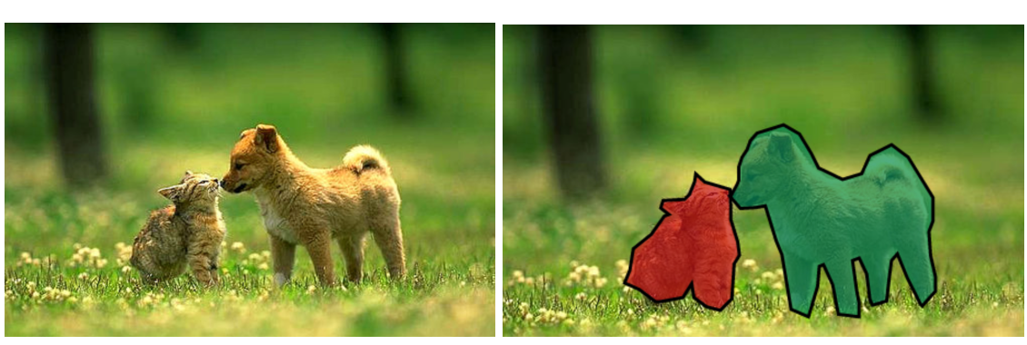
In lucid terms, segmentation is pixel classification. If an image has a cat and dog, we want the machine to identify the cat and dog pixels and flag them as 1(cat) or 2(dog) in the output. Every other pixel (background, noise, etc) is 0. To train such models, we use pairs of images and masks.
Let’s say you want to identify brain tumours in MRI scans. You’ll first create a training set of positive(tumour) and negative(non-tumour) images. For each, you’ll then create a corresponding mask. How’s that done? Take an MRI scan, locate the tumour region, convert all pixel values in that region to 0, and set all other pixels to 1. Naturally, non-tumour masks will be utter black. A model trained on these pairs (Input=MRI,Output=Mask) would operate to identify tumours in an MRI scan. Useful, isn’t it?

Now, let’s plunge deeper into the neural network architecture required for segmenting images.
Conventionally, CNNs are deft at identifying what’s present in an image. For segmentation, CNNs also need to learn to position image constituents precisely. UNet is equipped to do just that. The original UNet paper describes it as a network divided into two parts — contracting (encoder) and expansive (decoder). Let’s start with the encoder part (Note, I have made some minor modifications to the architecture presented in the UNet paper).
# Important Libraries to import
import pandas as pd
import numpy as np
import matplotlib.pyplot as plt
import os
import cv2
import tensorflow as tf
from tensorflow.keras import Input
from tensorflow.keras.models import Model, load_model, save_model
from tensorflow.keras.layers import Input, Activation, BatchNormalization, Lambda, Conv2D, Conv2DTranspose,MaxPooling2D, concatenate,UpSampling2D,Dropout
from tensorflow.keras.optimizers import Adam
from tensorflow.keras.callbacks import EarlyStopping, ModelCheckpoint,ReduceLROnPlateau
from tensorflow.keras import backend as K
from tensorflow.keras.preprocessing.image import ImageDataGenerator
from sklearn.model_selection import KFold
from tensorflow.keras.losses import BinaryCrossentropy
import random
2.1 Encoder
The encoder functions like a general CNN. It continually breaks down the input to discern features associated with the objects in an image. This process repeats in multiple blocks (encoder blocks). Each block consists of the following:
- Two convolutional layers with padding and (3,3) kernels in succession (we’ll call this a convolution block). One may also include batch normalisation/dropout layers wherever necessary [The original paper used unpadded convolutions]. We’ll use relu as activation function.
- A max-pooling layer with stride of 2 to squeeze the image down
# Functions to build the encoder path
def conv_block(inp, filters, padding='same', activation='relu'):
"""
Convolution block of a UNet encoder
"""
x = Conv2D(filters, (3, 3), padding=padding, activation=activation)(inp)
x = Conv2D(filters, (3, 3), padding=padding)(x)
x = BatchNormalization(axis=3)(x)
x = Activation(activation)(x)
return xdef encoder_block(inp, filters, padding='same', pool_stride=2,
activation='relu'):
"""
Encoder block of a UNet passes the result from the convolution block
above to a max pooling layer
"""
x = conv_block(inp, filters, padding, activation)
p = MaxPooling2D(pool_size=(2, 2), strides=pool_stride)(x)
return x, p
If you notice, the encoder_block returns two values- the image before and after max-pooling. UNet passes the latter (p) to the next block and stores the former (x) in memory. Why? We’ll expound on this later.
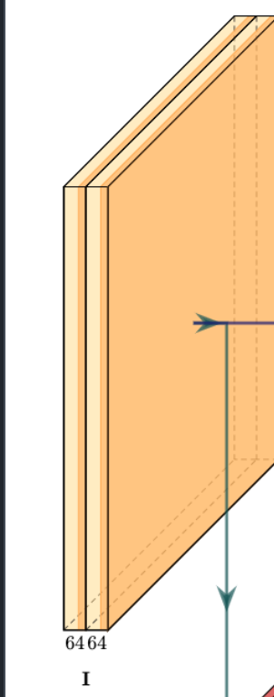
Above is a copy of the first encoder block described in the UNet paper. It comprises two convolutional layers with 64 filters applied sequentially followed by a max-pooling layer (indicated by the down-green arrow). We’ll replicate this with the above-discussed modifications. Input shape specification is not mandatory for networks like UNet that do not include a dense(flat) layer, yet, we’ll define the input shape as (256,256,1).
# Building the first block
inputs = Input((256,256,1))
d1,p1 = encoder_block(inputs,64)
This first block is followed by three more similar blocks having filters = 128,256,512. Together, the four blocks form the contraction path/encoder.
#Building the other four blocks
d2,p2 = encoder_block(p1,128)
d3,p3 = encoder_block(p2,256)
d4,p4 = encoder_block(p3,512)
1.2 MidSection
Yes, we discussed that the network had two parts, but I like to treat the middle component separately.

It takes the max-pooled output from the previous encoder block and runs it through two successive (3,3) convolutions of 1024 filters. Just like the convolution block, you ask? Yes, only this time, the output does not pass for max pooling. Ergo, we’ll use conv_block, instead of encoder_block, to create the middle section.
# Middle convolution block (no max pooling)
mid = conv_block(p4,1024) #Midsection
This final output will now be upsampled.
1.3 Decoder
Having mouldered the image into numerous feature maps, UNet has a fair idea of what’s in the input image. It knows the different classes (objects) the image contains. Now, it needs to predict the correct location of all these classes and label their pixels accordingly in the final output. To do so, UNet leverages two key ideas — skip connections and upsampling.
1.3.1 Transpose Convolution
After traversing down the encoder and going through the mid-block, the input transforms to shape (16,16,1024)[You can check this using the model.summary( ) api of keras]. UNet then applies transpose convolution to upsample the output. So what’s transposed convolution? See, if the image below answers your question.
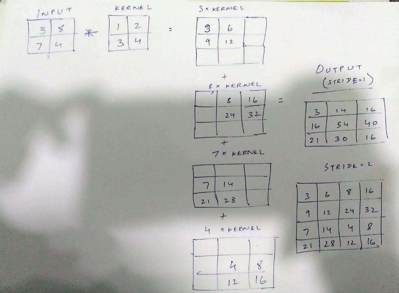
Essentially, we multiply the kernel weights by each entry in the input and stitch up all the (2,2) outputs to make the final output. At mutual indices, the numbers add up. Like convolution kernels, weights in transpose convolution kernels are also learnable. The network learns them during back-propagation to accurately upsample the feature maps. Refer this article to know more about transposed convolutions.
1.3.2 Skip Connections
For each encoder block, UNet also has a conjugate decoder block. We already discussed that decoder blocks learn to upsample the images. To enhance their learning and ensure that pixels are positioned correctly in the final output, decoders seek help from their corresponding encoders. They avail this in the form of skip connections.
Skip connections are the essence of UNet. If you’ve previously worked with resnets, you’d be familiar with this concept. In 1.1, we discussed that UNet stores the output (x) of the convolution block in memory. These outputs are concatenated with the upsampled images from each decoder block. Horizontal arrows in the image below represent the skip connections.

Researchers reckon that as input images roll deeper into a network, the finer details, such as the whereabouts of different objects/classes in an image, are lost. Skip connections transfer misplaced information from the initial layers enabling UNet to create better segmentation maps.
The concatenated, upsampled images then stream into convolution blocks (2 successive convolution layers). Hence, we use the following function to create the decoder blocks.
# Functions to build the decoder block
def decoder_block(inp,filters,concat_layer,padding='same'):
#Upsample the feature maps
x=Conv2DTranspose(filters,(2,2),strides=(2,2),padding=padding)(inp)
x=concatenate([x,concat_layer])#Concatenation/Skip conncetion with conjuagte encoder
x=conv_block(x,filters)#Passed into the convolution block above
return x
1.4 Final UNet Network
Below is our final UNet network. The output after e5 has shape (256,256,64). To match it to the input (256,256,1), we’ll use a (1,1) convolution layer with 1 filter. Do watch this Andrew Ng video if you are curious about 1,1 convolutions.
# Bulding the Unet model using the above functions
inputs=Input((256,256,1))
d1,p1=encoder_block(inputs,64)
d2,p2=encoder_block(p1,128)
d3,p3=encoder_block(p2,256)
d4,p4=encoder_block(p3,512)
mid=conv_block(p4,1024) #Midsection
e2=decoder_block(mid,512,d4) #Conjugate of encoder 4
e3=decoder_block(e2,256,d3) #Conjugate of encoder 3
e4=decoder_block(e3,128,d2) #Conjugate of encoder 2
e5=decoder_block(e4,64,d1) #Conjugate of encoder 1
outputs = Conv2D(1, (1,1),activation=None)(e5) #Final Output
ml=Model(inputs=[inputs],outputs=[outputs,o1],name='Unet')
2. Image Segmentation and deep supervision
Okay, time to implement what we’ve learnt.
We’ll perform image segmentation on this covid-19 chest x-ray (main dataset) database. It includes four image classes — Covid, Normal, Lung Opacity, and Viral Pneumonia. Through this post, I merely aim to share how one can use supervision loss and the Keras model subclass to segment images. Performance is not a factor here.
Hence, I’ll frame a simple problem. We’ll take images from the Covid class and segment their pixels into lungs and non-lungs. (Note we are not trying to train the model to identify covid affected regions but map the space occupied by lungs). Typically, however, medical imaging involves extremely complex cases like finding tumour-affected organs, etc. While we won’t deal with them here, you can use/modify the attached code for such compelling applications.
We use the following code block to retrieve image/mask paths from directory
# Block to read image paths, will be used in image data generator
df = pd.DataFrame(columns=['img_path','msk_path','img_shape','msk_shape','class'])
for cat in ['COVID']:
dir_ = f"../input/covid19-radiography-database/COVID-19_Radiography_Dataset/{cat}"
for f in os.listdir(f"{dir_}/images"):
s1 = cv2.imread(f"{dir_}/images/{f}",config.img_type_num).shape
s2 = cv2.imread(f"{dir_}/masks/{f}",config.msk_type_num).shape
dic={'img_path':f"{dir_}/images/{f}",'msk_path':f"{dir_}/masks/{f}",'img_shape':s1,
'msk_shape':s2}
df = df.append(dic,ignore_index=True)
Following are a few images and their corresponding masks from the dataset. The masks, as discussed, have two classes:
0: Lungs
1: Non-lungs

2.1 Loss function and deep supervision loss
The training masks have only two values, 0 and 1. Hence, we can use binary cross-entropy to calculate the loss between them and our final outputs. Now, let’s address the elephant in the room — supervision loss.
A problem with deep neural architectures is gradient loss. Some architectures are so deep that gradients vanish as they back-propagate to the initial layers, resulting in minimal weight shift in initial layers leading to deficient learning. Furthermore, it makes the model disproportionately reliant on deeper layers for performance.
To boost gradient flow this paper suggests calculating loss at different decoder levels. How exactly, you ask? Firstly, as shown below, we’ll extract an extra output ‘o1’ from the network. We’ll take the result from the second last decoder(e4), which is of shape (128,128,128), and shrink it down to (128,128,1) using (1,1) convolution filter.
# Adding output from 2nd last decoder block
inputs=Input((256,256,1))
d1,p1=encoder_block(inputs,64)
d2,p2=encoder_block(p1,128)
d3,p3=encoder_block(p2,256)
d4,p4=encoder_block(p3,512)
mid=conv_block(p4,1024) #Midsection
e2=decoder_block(mid,512,d4) #Conjugate of encoder 4
e3=decoder_block(e2,256,d3) #Conjugate of encoder 3
e4=decoder_block(e3,128,d2) #Conjugate of encoder 2
o1 = Conv2D(1,(1,1),activation=None)(e4) # Output from 2nd last decoder
e5=decoder_block(e4,64,d1) #Conjugate of encoder 1
outputs = Conv2D(1, (1,1),activation=None)(e5) #Final Output
Then, we’ll add o1 as a model output by appending to the output list in Keras’s model API.
# Adding output to output list in keras model API
ml=Model(inputs=[inputs],outputs=[outputs,o1],name='Unet')
Next, to calculate the loss from this level, we’ll also need to resize a copy of the input to (128,128,1). Now, the final loss will be:
We can also take a weighted combination of the two losses. Computing loss at different layers also equip them to produce a better approximation of the final output.
2.2 Training using Keras model subclass
Alright, all that remains now is training. While, technically you could pass a list of input and resized input in the renowned ‘ml.fit’, I prefer to use the keras model subclass. It permits us to play more with the loss function.
We create a class network with inheritance from tf.keras.Model. We’ll pass the model to be used(ml), loss function (binary cross entropy), metric (dice loss), and loss weights (to weight losses from the two decoder levels) while initialising object of class network.
# Defining network class which inherits keras model class
class network(tf.keras.Model):def __init__(self,model,loss,metric,loss_weights):
super().__init__()
self.loss = loss
self.metric = metric
self.model = model
self.loss_weights = loss_weights
Then we’ll override what happens in ‘ml.fit’ using the function train_step. The entire flow of input image through the network and loss computation is done under the scope of ‘tf.GradientTape’ which figures the gradients in just two lines.
# Overriding model.fit using def train_step
def call(self,inputs,training):
out = self.model(inputs)
if training==True:
return out
else:
if type(out) == list:
return out[0]
else:
return outdef calc_supervision_loss(self,y_true,y_preds):
loss = 0
for i,pred in enumerate(y_preds):
y_resized = tf.image.resize(y_true,[*pred.shape[1:3]])
loss+= self.loss_weights[i+1] * self.loss(y_resized,pred)
return loss
def train_step(self,data):
x,y = data
with tf.GradientTape() as tape:
y_preds = self(x,training=True)
if type(y_preds) == list:
loss = self.loss_weights[0] * self.loss(y,y_preds[0])
acc = self.metric(y,y_preds[0])
loss += self.calc_supervision_loss(y,y_preds[1:])
else:
loss = self.loss(y,y_preds)
acc = self.metric(y,y_preds)
trainable_vars = self.trainable_variables #Network trainable parameters
gradients = tape.gradient(loss, trainable_vars) #Calculating gradients
#Applying gradients to optimizer
self.optimizer.apply_gradients(zip(gradients, trainable_vars))
return loss,acc
When we operate with supervision loss, the network returns outputs in a list and we call the function calc_supervision_loss to compute the final loss.
Similarly, we can override the validation step
# Overriding validation step
def test_step(self,data):
x,y=data
y_pred = self(x,training=False)
loss = self.loss(y,y_pred)
acc = self.metric(y,y_pred)
return loss,acc
From here-on, things are customary. We’ll use Keras ImageDataGenerator to pass image-mask pairs for training.
# Keras Image data generator
def img_dataset(df_inp,path_img,path_mask,batch):
img_gen=ImageDataGenerator(rescale=1./255.)
df_img = img_gen.flow_from_dataframe(dataframe=df_inp,
x_col=path_img,
class_mode=None,
batch_size=batch,
color_mode=config.img_mode,
seed=config.seed,
target_size=config.img_size)
df_mask=img_gen.flow_from_dataframe(dataframe=df_inp,
x_col=path_mask,
class_mode=None,
batch_size=batch,
color_mode=config.msk_mode,
seed=config.seed,
target_size=config.img_size)
data_gen = zip(df_img,df_mask)
return data_gen
Next, we create training and validation sets, set the optimiser, instantiate the network class we created above and compile it. (As we inherit class network from keras, we can use .compile functionality directly)
train=img_dataset(train_ds,'img_path','msk_path',config.batch_size)
val=img_dataset(val_ds,'img_path','msk_path',config.batch_size)
opt = Adam(learning_rate=config.lr, epsilon=None, amsgrad=False,beta_1=0.9,beta_2=0.99)model = network(ml,BinaryCrossentropy(),dice_coef,[1,0.5])
model.compile(optimizer=opt,loss=BinaryCrossentropy(),metrics=[dice_coef])
Moving to the training loop
# Custom training loop
best_val = np.inf
for epoch in range(config.train_epochs):
epoch_train_loss = 0.0
epoch_train_acc=0.0
epoch_val_acc=0.0
epoch_val_loss=0.0
num_batches = 0
for x in train:
if num_batches > (len(train_ds)//config.batch_size):
break
a,b = model.train_step(x)
epoch_train_loss+=a
epoch_train_acc+=b
num_batches+=1
epoch_train_loss = epoch_train_loss/num_batches
epoch_train_acc = epoch_train_acc/num_batches
num_batches_v=0
for x in val:
if num_batches_v > (len(val_ds)//config.batch_size):
break
a,b = model.test_step(x)
epoch_val_loss+=a
epoch_val_acc+=b
num_batches_v+=1
epoch_val_loss=epoch_val_loss/num_batches_v
if epoch_val_loss < best_val:
best_val = epoch_val_loss
print('---Validation Loss improved,saving model---')
model.model.save('./weights',save_format='tf')
epoch_val_acc=epoch_val_acc/num_batches_v
template = ("Epoch: {}, TrainLoss: {}, TainAcc: {}, ValLoss: {}, ValAcc {}")
print(template.format(epoch,epoch_train_loss,epoch_train_acc,
epoch_val_loss,epoch_val_acc))
2.3 Results

The predicted masks are quite accurate. The model has a validation dice score of 0.96 and validation loss of 0.55. However, as discussed we should not read much into these values as the problem at hand was crude. The aim was to show how supervision loss can be used. In the paper referenced above, the authors used outputs from three decoders for calculating the final loss.
Deep CNNs used for segmentation often suffer from vanishing gradients. Can we combat this by calculating loss at different output levels?
Image segmentation entails partitioning image pixels into different classes. Some applications include identifying tumour regions in medical images, separating land and water areas in drone images, etc. Unlike classification, where CNNs output a class probability score vector, segmentation requires CNNs to output an image.

Accordingly, traditional CNN architectures are tweaked to yield the desired result. An array of architectures, including transformers, are available to segment images. But besides improving network design, researchers are constantly experimenting with other hacks to improve segmentation performance. Recently, I came across a work that briefly described the idea of calculating loss at multiple output levels (deep-supervision loss). In this post, I want to share the same.
We’ll implement a model similar to UNet, a commonly employed segmentation architecture, and train it with supervision loss using the Keras model subclass. You can refer to the attached Github/Kaggle links for code. I assume you’re familiar with the basics of Keras. As we have a lot to cover, I’ll link all all the resources and skip over a few things like dice-loss, keras training using model.fit, image generators, etc.
Let’s first start by understanding image segmentation.
In lucid terms, segmentation is pixel classification. If an image has a cat and dog, we want the machine to identify the cat and dog pixels and flag them as 1(cat) or 2(dog) in the output. Every other pixel (background, noise, etc) is 0. To train such models, we use pairs of images and masks.
Let’s say you want to identify brain tumours in MRI scans. You’ll first create a training set of positive(tumour) and negative(non-tumour) images. For each, you’ll then create a corresponding mask. How’s that done? Take an MRI scan, locate the tumour region, convert all pixel values in that region to 0, and set all other pixels to 1. Naturally, non-tumour masks will be utter black. A model trained on these pairs (Input=MRI,Output=Mask) would operate to identify tumours in an MRI scan. Useful, isn’t it?
Now, let’s plunge deeper into the neural network architecture required for segmenting images.
Conventionally, CNNs are deft at identifying what’s present in an image. For segmentation, CNNs also need to learn to position image constituents precisely. UNet is equipped to do just that. The original UNet paper describes it as a network divided into two parts — contracting (encoder) and expansive (decoder). Let’s start with the encoder part (Note, I have made some minor modifications to the architecture presented in the UNet paper).
# Important Libraries to import
import pandas as pd
import numpy as np
import matplotlib.pyplot as plt
import os
import cv2
import tensorflow as tf
from tensorflow.keras import Input
from tensorflow.keras.models import Model, load_model, save_model
from tensorflow.keras.layers import Input, Activation, BatchNormalization, Lambda, Conv2D, Conv2DTranspose,MaxPooling2D, concatenate,UpSampling2D,Dropout
from tensorflow.keras.optimizers import Adam
from tensorflow.keras.callbacks import EarlyStopping, ModelCheckpoint,ReduceLROnPlateau
from tensorflow.keras import backend as K
from tensorflow.keras.preprocessing.image import ImageDataGenerator
from sklearn.model_selection import KFold
from tensorflow.keras.losses import BinaryCrossentropy
import random
2.1 Encoder
The encoder functions like a general CNN. It continually breaks down the input to discern features associated with the objects in an image. This process repeats in multiple blocks (encoder blocks). Each block consists of the following:
- Two convolutional layers with padding and (3,3) kernels in succession (we’ll call this a convolution block). One may also include batch normalisation/dropout layers wherever necessary [The original paper used unpadded convolutions]. We’ll use relu as activation function.
- A max-pooling layer with stride of 2 to squeeze the image down
# Functions to build the encoder path
def conv_block(inp, filters, padding='same', activation='relu'):
"""
Convolution block of a UNet encoder
"""
x = Conv2D(filters, (3, 3), padding=padding, activation=activation)(inp)
x = Conv2D(filters, (3, 3), padding=padding)(x)
x = BatchNormalization(axis=3)(x)
x = Activation(activation)(x)
return xdef encoder_block(inp, filters, padding='same', pool_stride=2,
activation='relu'):
"""
Encoder block of a UNet passes the result from the convolution block
above to a max pooling layer
"""
x = conv_block(inp, filters, padding, activation)
p = MaxPooling2D(pool_size=(2, 2), strides=pool_stride)(x)
return x, p
If you notice, the encoder_block returns two values- the image before and after max-pooling. UNet passes the latter (p) to the next block and stores the former (x) in memory. Why? We’ll expound on this later.
Above is a copy of the first encoder block described in the UNet paper. It comprises two convolutional layers with 64 filters applied sequentially followed by a max-pooling layer (indicated by the down-green arrow). We’ll replicate this with the above-discussed modifications. Input shape specification is not mandatory for networks like UNet that do not include a dense(flat) layer, yet, we’ll define the input shape as (256,256,1).
# Building the first block
inputs = Input((256,256,1))
d1,p1 = encoder_block(inputs,64)
This first block is followed by three more similar blocks having filters = 128,256,512. Together, the four blocks form the contraction path/encoder.
#Building the other four blocks
d2,p2 = encoder_block(p1,128)
d3,p3 = encoder_block(p2,256)
d4,p4 = encoder_block(p3,512)
1.2 MidSection
Yes, we discussed that the network had two parts, but I like to treat the middle component separately.
It takes the max-pooled output from the previous encoder block and runs it through two successive (3,3) convolutions of 1024 filters. Just like the convolution block, you ask? Yes, only this time, the output does not pass for max pooling. Ergo, we’ll use conv_block, instead of encoder_block, to create the middle section.
# Middle convolution block (no max pooling)
mid = conv_block(p4,1024) #Midsection
This final output will now be upsampled.
1.3 Decoder
Having mouldered the image into numerous feature maps, UNet has a fair idea of what’s in the input image. It knows the different classes (objects) the image contains. Now, it needs to predict the correct location of all these classes and label their pixels accordingly in the final output. To do so, UNet leverages two key ideas — skip connections and upsampling.
1.3.1 Transpose Convolution
After traversing down the encoder and going through the mid-block, the input transforms to shape (16,16,1024)[You can check this using the model.summary( ) api of keras]. UNet then applies transpose convolution to upsample the output. So what’s transposed convolution? See, if the image below answers your question.
Essentially, we multiply the kernel weights by each entry in the input and stitch up all the (2,2) outputs to make the final output. At mutual indices, the numbers add up. Like convolution kernels, weights in transpose convolution kernels are also learnable. The network learns them during back-propagation to accurately upsample the feature maps. Refer this article to know more about transposed convolutions.
1.3.2 Skip Connections
For each encoder block, UNet also has a conjugate decoder block. We already discussed that decoder blocks learn to upsample the images. To enhance their learning and ensure that pixels are positioned correctly in the final output, decoders seek help from their corresponding encoders. They avail this in the form of skip connections.
Skip connections are the essence of UNet. If you’ve previously worked with resnets, you’d be familiar with this concept. In 1.1, we discussed that UNet stores the output (x) of the convolution block in memory. These outputs are concatenated with the upsampled images from each decoder block. Horizontal arrows in the image below represent the skip connections.
Researchers reckon that as input images roll deeper into a network, the finer details, such as the whereabouts of different objects/classes in an image, are lost. Skip connections transfer misplaced information from the initial layers enabling UNet to create better segmentation maps.
The concatenated, upsampled images then stream into convolution blocks (2 successive convolution layers). Hence, we use the following function to create the decoder blocks.
# Functions to build the decoder block
def decoder_block(inp,filters,concat_layer,padding='same'):
#Upsample the feature maps
x=Conv2DTranspose(filters,(2,2),strides=(2,2),padding=padding)(inp)
x=concatenate([x,concat_layer])#Concatenation/Skip conncetion with conjuagte encoder
x=conv_block(x,filters)#Passed into the convolution block above
return x
1.4 Final UNet Network
Below is our final UNet network. The output after e5 has shape (256,256,64). To match it to the input (256,256,1), we’ll use a (1,1) convolution layer with 1 filter. Do watch this Andrew Ng video if you are curious about 1,1 convolutions.
# Bulding the Unet model using the above functions
inputs=Input((256,256,1))
d1,p1=encoder_block(inputs,64)
d2,p2=encoder_block(p1,128)
d3,p3=encoder_block(p2,256)
d4,p4=encoder_block(p3,512)
mid=conv_block(p4,1024) #Midsection
e2=decoder_block(mid,512,d4) #Conjugate of encoder 4
e3=decoder_block(e2,256,d3) #Conjugate of encoder 3
e4=decoder_block(e3,128,d2) #Conjugate of encoder 2
e5=decoder_block(e4,64,d1) #Conjugate of encoder 1
outputs = Conv2D(1, (1,1),activation=None)(e5) #Final Output
ml=Model(inputs=[inputs],outputs=[outputs,o1],name='Unet')
2. Image Segmentation and deep supervision
Okay, time to implement what we’ve learnt.
We’ll perform image segmentation on this covid-19 chest x-ray (main dataset) database. It includes four image classes — Covid, Normal, Lung Opacity, and Viral Pneumonia. Through this post, I merely aim to share how one can use supervision loss and the Keras model subclass to segment images. Performance is not a factor here.
Hence, I’ll frame a simple problem. We’ll take images from the Covid class and segment their pixels into lungs and non-lungs. (Note we are not trying to train the model to identify covid affected regions but map the space occupied by lungs). Typically, however, medical imaging involves extremely complex cases like finding tumour-affected organs, etc. While we won’t deal with them here, you can use/modify the attached code for such compelling applications.
We use the following code block to retrieve image/mask paths from directory
# Block to read image paths, will be used in image data generator
df = pd.DataFrame(columns=['img_path','msk_path','img_shape','msk_shape','class'])
for cat in ['COVID']:
dir_ = f"../input/covid19-radiography-database/COVID-19_Radiography_Dataset/{cat}"
for f in os.listdir(f"{dir_}/images"):
s1 = cv2.imread(f"{dir_}/images/{f}",config.img_type_num).shape
s2 = cv2.imread(f"{dir_}/masks/{f}",config.msk_type_num).shape
dic={'img_path':f"{dir_}/images/{f}",'msk_path':f"{dir_}/masks/{f}",'img_shape':s1,
'msk_shape':s2}
df = df.append(dic,ignore_index=True)
Following are a few images and their corresponding masks from the dataset. The masks, as discussed, have two classes:
0: Lungs
1: Non-lungs
2.1 Loss function and deep supervision loss
The training masks have only two values, 0 and 1. Hence, we can use binary cross-entropy to calculate the loss between them and our final outputs. Now, let’s address the elephant in the room — supervision loss.
A problem with deep neural architectures is gradient loss. Some architectures are so deep that gradients vanish as they back-propagate to the initial layers, resulting in minimal weight shift in initial layers leading to deficient learning. Furthermore, it makes the model disproportionately reliant on deeper layers for performance.
To boost gradient flow this paper suggests calculating loss at different decoder levels. How exactly, you ask? Firstly, as shown below, we’ll extract an extra output ‘o1’ from the network. We’ll take the result from the second last decoder(e4), which is of shape (128,128,128), and shrink it down to (128,128,1) using (1,1) convolution filter.
# Adding output from 2nd last decoder block
inputs=Input((256,256,1))
d1,p1=encoder_block(inputs,64)
d2,p2=encoder_block(p1,128)
d3,p3=encoder_block(p2,256)
d4,p4=encoder_block(p3,512)
mid=conv_block(p4,1024) #Midsection
e2=decoder_block(mid,512,d4) #Conjugate of encoder 4
e3=decoder_block(e2,256,d3) #Conjugate of encoder 3
e4=decoder_block(e3,128,d2) #Conjugate of encoder 2
o1 = Conv2D(1,(1,1),activation=None)(e4) # Output from 2nd last decoder
e5=decoder_block(e4,64,d1) #Conjugate of encoder 1
outputs = Conv2D(1, (1,1),activation=None)(e5) #Final Output
Then, we’ll add o1 as a model output by appending to the output list in Keras’s model API.
# Adding output to output list in keras model API
ml=Model(inputs=[inputs],outputs=[outputs,o1],name='Unet')
Next, to calculate the loss from this level, we’ll also need to resize a copy of the input to (128,128,1). Now, the final loss will be:
We can also take a weighted combination of the two losses. Computing loss at different layers also equip them to produce a better approximation of the final output.
2.2 Training using Keras model subclass
Alright, all that remains now is training. While, technically you could pass a list of input and resized input in the renowned ‘ml.fit’, I prefer to use the keras model subclass. It permits us to play more with the loss function.
We create a class network with inheritance from tf.keras.Model. We’ll pass the model to be used(ml), loss function (binary cross entropy), metric (dice loss), and loss weights (to weight losses from the two decoder levels) while initialising object of class network.
# Defining network class which inherits keras model class
class network(tf.keras.Model):def __init__(self,model,loss,metric,loss_weights):
super().__init__()
self.loss = loss
self.metric = metric
self.model = model
self.loss_weights = loss_weights
Then we’ll override what happens in ‘ml.fit’ using the function train_step. The entire flow of input image through the network and loss computation is done under the scope of ‘tf.GradientTape’ which figures the gradients in just two lines.
# Overriding model.fit using def train_step
def call(self,inputs,training):
out = self.model(inputs)
if training==True:
return out
else:
if type(out) == list:
return out[0]
else:
return outdef calc_supervision_loss(self,y_true,y_preds):
loss = 0
for i,pred in enumerate(y_preds):
y_resized = tf.image.resize(y_true,[*pred.shape[1:3]])
loss+= self.loss_weights[i+1] * self.loss(y_resized,pred)
return loss
def train_step(self,data):
x,y = data
with tf.GradientTape() as tape:
y_preds = self(x,training=True)
if type(y_preds) == list:
loss = self.loss_weights[0] * self.loss(y,y_preds[0])
acc = self.metric(y,y_preds[0])
loss += self.calc_supervision_loss(y,y_preds[1:])
else:
loss = self.loss(y,y_preds)
acc = self.metric(y,y_preds)
trainable_vars = self.trainable_variables #Network trainable parameters
gradients = tape.gradient(loss, trainable_vars) #Calculating gradients
#Applying gradients to optimizer
self.optimizer.apply_gradients(zip(gradients, trainable_vars))
return loss,acc
When we operate with supervision loss, the network returns outputs in a list and we call the function calc_supervision_loss to compute the final loss.
Similarly, we can override the validation step
# Overriding validation step
def test_step(self,data):
x,y=data
y_pred = self(x,training=False)
loss = self.loss(y,y_pred)
acc = self.metric(y,y_pred)
return loss,acc
From here-on, things are customary. We’ll use Keras ImageDataGenerator to pass image-mask pairs for training.
# Keras Image data generator
def img_dataset(df_inp,path_img,path_mask,batch):
img_gen=ImageDataGenerator(rescale=1./255.)
df_img = img_gen.flow_from_dataframe(dataframe=df_inp,
x_col=path_img,
class_mode=None,
batch_size=batch,
color_mode=config.img_mode,
seed=config.seed,
target_size=config.img_size)
df_mask=img_gen.flow_from_dataframe(dataframe=df_inp,
x_col=path_mask,
class_mode=None,
batch_size=batch,
color_mode=config.msk_mode,
seed=config.seed,
target_size=config.img_size)
data_gen = zip(df_img,df_mask)
return data_gen
Next, we create training and validation sets, set the optimiser, instantiate the network class we created above and compile it. (As we inherit class network from keras, we can use .compile functionality directly)
train=img_dataset(train_ds,'img_path','msk_path',config.batch_size)
val=img_dataset(val_ds,'img_path','msk_path',config.batch_size)
opt = Adam(learning_rate=config.lr, epsilon=None, amsgrad=False,beta_1=0.9,beta_2=0.99)model = network(ml,BinaryCrossentropy(),dice_coef,[1,0.5])
model.compile(optimizer=opt,loss=BinaryCrossentropy(),metrics=[dice_coef])
Moving to the training loop
# Custom training loop
best_val = np.inf
for epoch in range(config.train_epochs):
epoch_train_loss = 0.0
epoch_train_acc=0.0
epoch_val_acc=0.0
epoch_val_loss=0.0
num_batches = 0
for x in train:
if num_batches > (len(train_ds)//config.batch_size):
break
a,b = model.train_step(x)
epoch_train_loss+=a
epoch_train_acc+=b
num_batches+=1
epoch_train_loss = epoch_train_loss/num_batches
epoch_train_acc = epoch_train_acc/num_batches
num_batches_v=0
for x in val:
if num_batches_v > (len(val_ds)//config.batch_size):
break
a,b = model.test_step(x)
epoch_val_loss+=a
epoch_val_acc+=b
num_batches_v+=1
epoch_val_loss=epoch_val_loss/num_batches_v
if epoch_val_loss < best_val:
best_val = epoch_val_loss
print('---Validation Loss improved,saving model---')
model.model.save('./weights',save_format='tf')
epoch_val_acc=epoch_val_acc/num_batches_v
template = ("Epoch: {}, TrainLoss: {}, TainAcc: {}, ValLoss: {}, ValAcc {}")
print(template.format(epoch,epoch_train_loss,epoch_train_acc,
epoch_val_loss,epoch_val_acc))
2.3 Results
The predicted masks are quite accurate. The model has a validation dice score of 0.96 and validation loss of 0.55. However, as discussed we should not read much into these values as the problem at hand was crude. The aim was to show how supervision loss can be used. In the paper referenced above, the authors used outputs from three decoders for calculating the final loss.
Denial of responsibility! Techno Blender is an automatic aggregator of the all world’s media. In each content, the hyperlink to the primary source is specified. All trademarks belong to their rightful owners, all materials to their authors. If you are the owner of the content and do not want us to publish your materials, please contact us by email – [email protected]. The content will be deleted within 24 hours.