
Implementation Details Of Reluplex: An Efficient SMT Solver for Verifying Deep Neural Networks
How to formally verify the bounds of your Neural Network
Reluplex is an algorithm submitted to CAV in 2017 by Stanford University [1]. Reluplex accepts as input a neural network and a set of constraints on the inputs and outputs of the network. The network must be composed of only linear layers and ReLU activations. The bounds may restrict any arbitrary number of input or output nodes to a single value or a range of values. The algorithm then finds an input within the given input bounds that can produce an output within the given output bounds. If no example exists, it will determine that the problem is infeasible in a reasonable amount of time.
Algorithm Uses
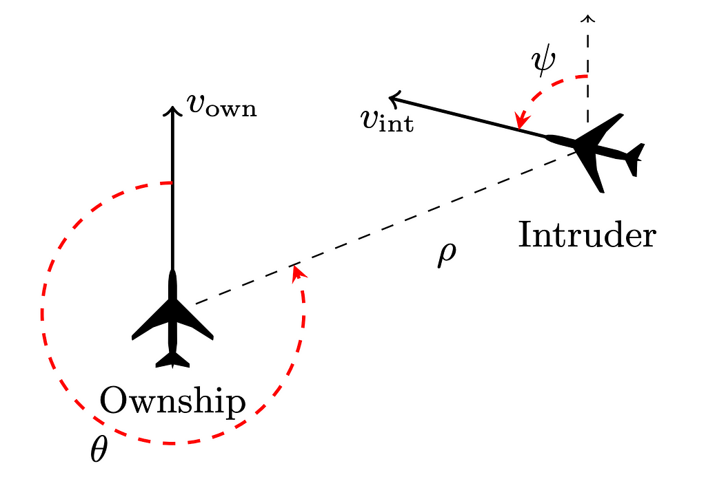
The original algorithm was written to help build the “Airborne Collision-Avoidance System for drone” system. This system uses 45 deep learning networks to fly a series of drones. The researches needed a way to formally gurante that regardless of what other inputs their networks are receiving that if two drones got too close to each other they will always fly away from each other and not crash. In the most extreme case, the algorithm was able to complete these verifications within 109.6 hours, which while a long time is still an order of magnitude faster than the previous state of the art algorithm.
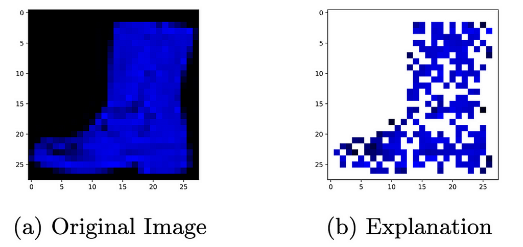
In a more recent publication, Marabou [4] (a new state of the art version of reluplex) has been used for neural network explainability. The algorithm works by finding an upper bound and a lower bound for the for what parts of the input are strictly necessary to produce output that a network generates. [6]
The algorithm has also been used to set precise bounds on what adversarial perturbations are large enough to change the output of a network.
Basic Neural Network
Before explaining the details of this algorithm, we first need to cover some basics of neural networks. Here is a simple diagram of a network:
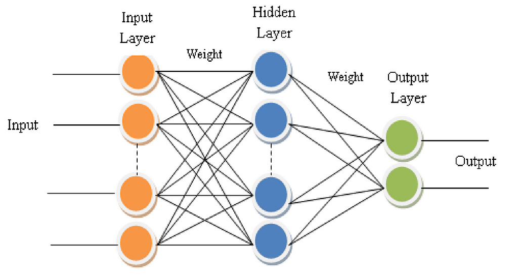
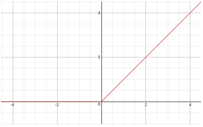
In the diagram above, the hidden layer is calculated by multiplying all of the nodes in a previous layer by a specific value, then adding them together, and then adding a bias term that is specific to each node to this sum. The summed value then goes through an activation function f before being used in the next layer. The activation function we will be using in this article is the ReLU function which is defined as f(x) = x if x > 0 else 0:
High Level View Of Reluplex
What reluplex does is it tries to put a neural network into a simplex problem. Once constraints are set inside of a simplex problem, it is guaranteed to be able to find a solution quickly or determine if there is no valid point given the constraints. It is also an algorithm that has proven to be exceptionally efficient at doing thisand there are reputable formal proofs that guarantee it will work every single time. This is exactly what we want for our reluplex problem. The only problem is that reluplex can only work with linear constraints, and the relu funtions in our neural network are non-linear and can not be directly put into the simplex method. To make it linear, must be done then is to choose to impose the constraint that either the input to the relu must be non-positive and make the relu inactive, or the input of the relu must be constrained to be non-negative making the relu function active. By default, most SMT solvers would get around this by manually checking every possible combination of constraint. However, in a network with 300 plus relu functions this can turn into 2³⁰⁰ case splits which is impracticably slow to solve. What reluplex does then is it first encodes everything it can about a network without the reluconstraints and finds a feasible point. If a feasible point exists, it will then fix the parts of a network that violate the relu constraint one at a time. If a specific node is updated too many times will split the problem into one case where that node is always active and another case where it’s always inactive then continue the search. The original authors of the paper are able to formally prove that this algorithm is sound and complete and will terminate in a finite amount of steps. They also empirically show that it terminates much faster than a simple brute force approach of checking every single possible case.
Purpose Of This Article
The original paper gives a good example of the algorithm actually works. However, they assume the reader has a deep understanding of how the simplex method works and they skip over some important design choices that have to be made. The purpose of this article then is to carefully lay out the exact steps the algorithm uses with all the details of how the simplex method works. We also provide a simplified and working implementation of the algorithm in python. The original paper provides formal proofs to guarantee that as long as the simplex method works, reluplex will work. There is also a relatively large body of publications that prove that reluplex works. As such, we do not provide any formal justification on why this algorithm works. We simply wish to explain the steps needed for the algorithm and give an intuition of why the authors choose those steps. Deeply understanding this algorithm may require reading the original reluplex paper or studying the simplex method.
The Simplex Method
The simplex method is designed to address optimization problems within a defined space. These problems involve a set of non-negative variables, the introduction of constraints on those variables, and the declaration of an objective function.
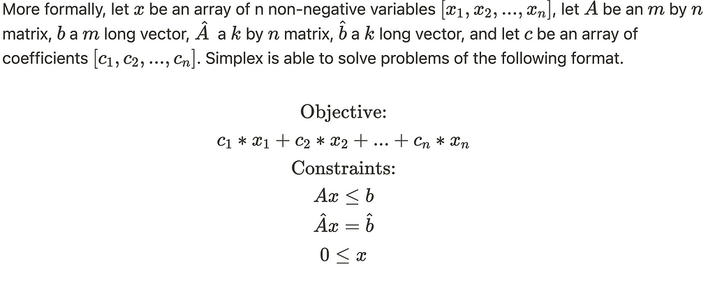
After establishing these constraints, the simplex method initially verifies the existence of a point that satisfies the specified constraints. Upon identifying such a point, the method proceeds to find the point that maximizes the objective within the given constraints.
A Full Example Of Reluplex
The following is a basic neural network we will be using to demonstrate the full algorithm.
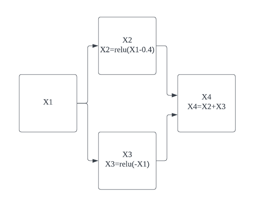
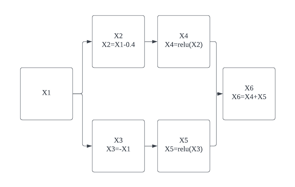
The first thing we need to do is break the hidden layer nodes, one node will be a linear function of the previous nodes, and the other node will a ReLU of the output of that linear function.
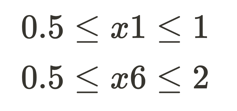
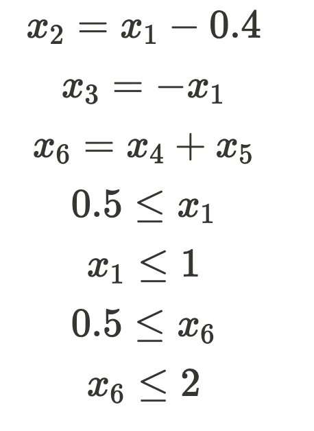
Now we declare the following bounds on our function input and output:
Given the model setup and declared constraints, our objective is to transform this problem into a simplex problem. Since the simplex method is limited to linear operations, directly incorporating a ReLU constraint into the setup is not feasible. However, we can introduce constraints for all other components of the network. If a solution is feasible without the ReLU constraints, we can systematically add these constraints one by one until we either discover a feasible solution or establish that the ReLU constraints render the problem impossible. Therefore, by encoding the applicable constraints, we now have the following:
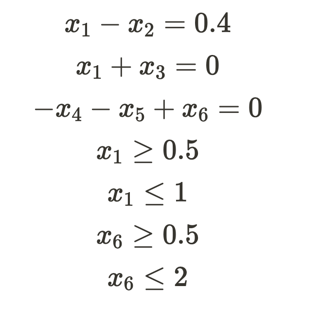
To incorporate these constraints into the simplex method, we need to convert them to standard form. In standard form, all non-constant variables are on the left-hand side, and all constants are on the right, with the constants being positive. Upon rewriting, we obtain the following:
Setting Up The Simplex Tableau
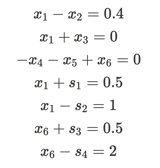
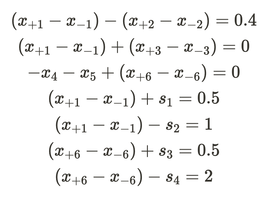
The subsequent step involves converting all inequalities into equality constraints. To achieve this, we will introduce slack variables. These variables are inherently non-negative and can assume arbitrarily large values. Additionally, they ensure that our new equality constraints are mathematically equivalent to our original inequality constraints.
Currently, the simplex method inherently accommodates only non-negative variables. However, the nodes in our network might not adhere to this non-negativity constraint. To accommodate negative values, we must substitute variables that can be either positive or negative with separate positive and negative variables, as illustrated below:
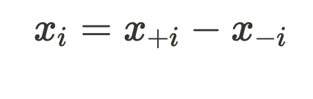
With this substitution, x_{+i} and x_{-i} can always be positive values but still combine together to make x_i to be negative. x_4 and x_5 come after a ReLU and as such are always non-negative and don’t need this substitution. However, all the other neural network node variables do. Doing these substitutions, we now have the following set of constraints.
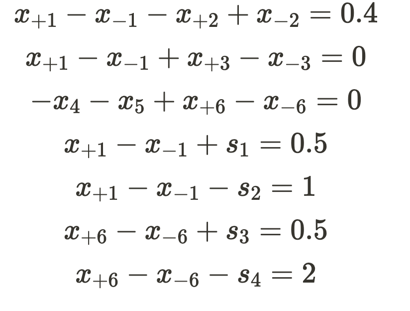
Distributing the negatives and removing the parenthesis we have the following:
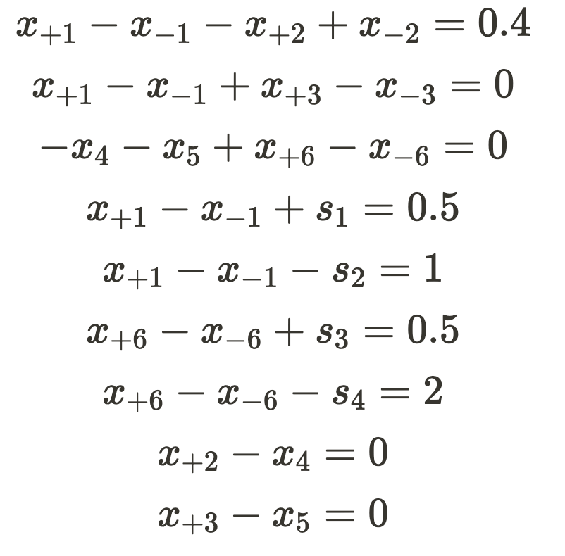
Now that we have separated variables into positive and negative parts, we need to take a small step back and remember that after we solve for this system of equations we will be needing to be making adjustments to fix the ReLU violations. To help make fixing ReLU violations easier, we are ready to introduce a new linear constraint. The constraint constraints we wish to add are setting x_{+2} = x_4 and x_{+3} = x_5. This will make it possible for both i in {2,3}, x_{+i} and x_{-i} may both me non-negative and when that happens the ReLU constraint will not be held. However, fixing the ReLU constraint will become as easy as adding a constraint to either make x_{+i} or x_{-i} equal zero. This will result in the following new set of constraints.
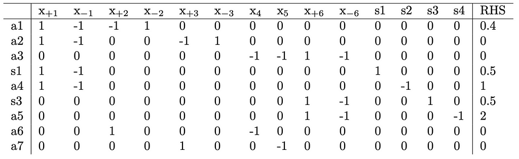
The clutter of having so many different variables around can make it hard to tell what’s going on. As such, we’ll rewrite everything into a tableau matrix.
Solving The Primal Problem
Now that we’ve transformed our problem into a tableau matrix, we will use the two-phase method to solve this setup. The first phase involves finding a feasible point, while the second phase moves the feasible point to maximize a specific utility function. However, for our specific use case, we don’t have a utility function; our goal is solely to determine the existence of a feasible point. Consequently, we will only execute the first phase of the two-phase method.
To identify a feasible point, the simplex method initially checks if setting all slack variables to the right-hand side and all other variables to zero is feasible. In our case, this approach is not viable due to non-zero equality constraints lacking a slack variable. Additionally, on lines 5 and 7, the slack variable is multiplied by a negative number, making it impossible for the expression to evaluate to positive right-hand sides, as slack variables are always positive. Therefore, to obtain an initial feasible point, we will introduce new auxiliary variables assigned to be equal to the right-hand side, setting all other variables to zero. This won’t be done for constraints with positive signed slack variables, as those slack variables may already equal the right-hand side. To enhance clarity, we will add a column on the left indicating which variables are assigned a non-zero value; these are referred to as our basic variables.
Our feasible point then is
It’s important to recognize that these auxiliary variables alter the solution, and in order to arrive at our desired true solution we need to eliminate them. To eliminate them, we will introduce an objective function to set them to zero. Specifically, we aim to minimize the function. a1 + a2 + a3 + a4 + a5 + a6 + a7. If we successfully minimize this function to zero, we can conclude that our original set of equations has a feasible point. However, if we are unable to achieve this, it indicates that there is no feasible point, allowing us to terminate the problem.
With the tableau and objective function declared, we are prepared to execute the pivots necessary to optimize our objective. The steps for doing which are as follows:
- Replace basic variables in objective function with non-basic variables. In this case, all the auxiliary variables are basic variables. To replace them, we pivot on all of the auxiliary columns and the rows that have a non-zero value entry for the basic variable. A pivot is done by adding or subtracting from the pivot row to all other rows until the only non-zero entry in the pivot column is the entry in the pivot row.
- Select a pivot column by finding the column with the first and largest value in the objective function.
- Select a pivot row by using bland’s rule. Bland’s rule we identify all positive entries in our column, divide the objective by those entries, and choose the row that yields the smallest value.
- Repeat steps 2 and 3 until all entries in the objective function are non-positive.
Once this done, we will have the following new tableau.
From this, we arrive at the point
We have successfully adjusted all of the auxiliary variables to equal zero. We also have pivoted away from them to make them all non-basic. Also, we will note that these values do indeed satisfy our initial linear constraints. As such, we no longer need the auxiliary variables may remove them from our set of linear equations. If we collapse the positive and negative variables and remove the auxilary variables we have this new point:

Relu Fix Search Procedure
By adding the constraints x_{+2} = x_4 and x_{+3} = x_5 we make it possible for both x_{+2} and x_{-2} to both be non-zero (same applies for x_{+3} and x_{-3} ). As can be seen above, both x_{+2} and x_{-2} are non-zero and relu(x_2) does not equal x_4. To fix the ReLU, there is no way to directly constrain simplex to either have x_{+2} or x_{-2} be zero, we must choose one case and create a constraint for that case. Choosing between these two cases is equivalent to deciding whether the ReLU will be in an active or inactive state. In the original paper, the authors address ReLU violations by assigning one side to equal the value of the other side at that specific moment. We believe this approach overly constrains the problem. That is because limiting the ReLU to a specific value and necessitating potentially an infinite number of configurations to check. Our solution, on the other hand, constrains the ReLU to be either active or inactive. Consequently, we only need to check these situations to cover the space of all allowable configurations.
As we need to decide whether the ReLU constraints are active or inactive, and with 2 to the n valid constraints to set, manually examining all possible configurations in a large network becomes impractical.
The authors of Reluplex propose addressing violations by attempting to solve them one ReLU fix at a time. They iteratively add one constraint to fix one specific violation, update the tableau to accomodate the new constraint, remove the constraint, then repeat for all other or new violations. Because only one constraint is ever in place it is possible that updating one ReLU fix can break one in another place that was already fixed. This can lead to a cycle of repeatedly fixing the same ReLU constraints. To get around this, if a ReLU node is updated five times, a “ReLU split” is executed. This split divides the problem into two cases: in one, they enforce that the negative side of the variable is zero, and in the other, the positive side is set to zero. Importantly, the constraint is not removed in either case, ensuring that the particular ReLU will never need fixing again. This allows the algorithm to only split on particularly “problematic” ReLU nodes, and empirical evidence shows that typically only about 10% of ReLUs need to split. Consequently, although some fixing operations may be repeated, the overall procedure remains faster than a simple brute-force check for every possibility.
Adding Constraint To Fix Relu
To address the ReLU violation, we need to constrain either x_{+2} or x_{-2} to be zero. To maintain a systematic approach, we will consistently attempt to set the positive variable to zero first. If that proves infeasible, we will then set the negative side to zero.
Introducing a new constraint involves adding a new auxiliary variable. If we add this variable and impose a constraint to set x_{+2}=0, the tableau is transformed as follows:
x_{+2} functions as a basic variable and appears in two distinct rows. This contradicts one of the assumptions necessary for the simplex method to function properly. Consequently, a quick pivot on (x_{+2}, x_{+2}) is necessary to rectify this issue. Executing this pivot yields the following:
Solving The Dual Problem
In the previous step, we applied the two-phase method to solve the last tableau. This method involves introducing artificial variables until a guaranteed trivial initial point is established. Subsequently, it pivots from one feasible point to another until an optimal solution is attained. However, instead of continuing with the two-phase method for this tableau, we will employ the dual simplex method.
The dual simplex method initiates by identifying a point that is optimally positioned beyond the given constraints, often referred to as a super-optimal point. It then progresses from one super-optimal point to another until it reaches a feasible point. Once a feasible point is reached, it is ensured to be the global optimal point. This method suits our current scenario as it enables us to add a constraint to our already solved tableau without the need to solve a primal problem. Given that we lack an inherent objective function, we will assign an objective function as follows:

Solving the Primal Problem typically involves transposing the matrix and replacing the objective function values with the right-hand side values. However, in this case, we can directly solve it using the tableau we’ve already set up. The process is as follows:
Applying this procedure to the problem we’ve established will reveal its infeasibility. This aligns with expectations since setting x_{+3} to zero would necessitate setting x_{+1}-x_{-1} or x_1 to 0.4 or lower, falling below the lower bound constraint of 0.5 we initially imposed on x_1.
Setting x_{-1}=0
Since setting x_{+1}=0 failed, we move on to trying to set x_{-1}=0. This actually will succeed and result in the following completed tableau:
From this, we have the new solution point:
Which if we collapse becomes:
Now that we have successfully made x_4 = relu(x_2) , we must remove the temporary constraint before we continuing.
Removing The Temporary ReLU Constraint
To lift the constraint, a pivot operation is required to explicitly state the constraint within a single row. This can be achieved by pivoting on our new a_1 column. Following Bland’s rule for selecting the pivot row, we identify all positive entries in our column, divide the objective by those entries, and choose the row that yields the smallest value. In this instance, the x_{-2} row emerges as the optimal choice since 0/1=0 is smaller than all other candidates. After performing the pivot, the resulting tableau is as follows:
It’s important to observe that none of the variable values have been altered. We can now confidently eliminate both the a_1 row and a_1 column from the tableau. This action effectively removes the constraint x_{-2}=0, resulting in the following updated tableau:
Continuing to Relu Split
As evident, we successfully addressed the ReLU violation, achieving the desired outcome of x_4 = ReLU(x_2). However, a new violation arises as x_5 does not equal ReLU(x_3). To fix this new violation, we follow the exact same procedure we used to fix the x_4 does not equal ReLU(x_2) violation. Once this is done though, we find that the tableau reverts to its state before we fixed x_4 = ReLU(x_2). If we continue, we will cycle between fixing x_4 = ReLU(x_2) and x_5 = ReLU(x_3) until we have updated one of these enough for a ReLU split to be triggered. This split creates two tableaus: one where x_{+2}=0 (shown to be infeasible) and another where x_{-2}=0, resulting in a tableau we have encountered before.
This time though, we will proceed without removing the constraint x_{-2}=0. Trying to fix the x_{+3}=0 constraint will be successful and result in the following values:
Which when we collapse becomes:

This outcome is free of ReLU violations and represents a valid point that the neural network can produce within the initially declared bounds. With this, our search concludes, and we can officially declare it complete.
Possible Optimizations
A significant optimization opportunity lies in cases where only one side of the ReLU is feasible. In such instances, it is unnecessary to remove the constraint. This is because, in those scenarios, we are not imposing any additional constraints, allowing us to conclude that if a side is infeasible, it will remain so indefinitely, regardless of additional constraints. Therefore, there is no need to remove the constraint on the feasible side. In our toy example, this optimization would have reduced the required updates from 13 to only 3. However, it’s important to note that we shouldn’t necessarily expect a proportionate improvement in larger networks. This optimization is used in our python implementation.
The original paper suggests other optimizations such as bound tightening, derived bounds, conflict analysis, and floating-point arithmetic. However, these optimizations are not implemented in our solution.
Code Implementations
For the best-performing and production-ready version of the algorithm, we suggest exploring the official Marabou GitHub page[5]. Additionally, you can delve into the official Reluplex repository for a more in-depth understanding of the algorithm[2]. The author has written a simplified implementation of ReLuPlex in Python[3]. This implementation can be valuable for grasping the algorithm and can serve as a foundation for developing a customized Python version of the algorithm.
References
[1][1702.01135] Reluplex: An Efficient SMT Solver for Verifying Deep Neural Networks (arxiv.org)
[2][1803.08375] Deep Learning using Rectified Linear Units (ReLU)
[2] Official Implementation of ReluPlex (github.com)
[3] Python Implementation of ReluPlex by author (github.com)
[4][1910.14574] An Abstraction-Based Framework for Neural Network Verification (arxiv.org)
[5] Official Implementation Of Marabou (github.com)
[6][2210.13915]Towards Formal XAI: Formally Approximate Minimal Explanations of Neural Networks
[7] Neural Networks By Science Direct
[8]Comprehensive Overview of Backpropagation Algorithm for Digital Image Denoising
Implementation Details Of Reluplex: An Efficient SMT Solver for Verifying Deep Neural Networks was originally published in Towards Data Science on Medium, where people are continuing the conversation by highlighting and responding to this story.
How to formally verify the bounds of your Neural Network

Reluplex is an algorithm submitted to CAV in 2017 by Stanford University [1]. Reluplex accepts as input a neural network and a set of constraints on the inputs and outputs of the network. The network must be composed of only linear layers and ReLU activations. The bounds may restrict any arbitrary number of input or output nodes to a single value or a range of values. The algorithm then finds an input within the given input bounds that can produce an output within the given output bounds. If no example exists, it will determine that the problem is infeasible in a reasonable amount of time.
Algorithm Uses
The original algorithm was written to help build the “Airborne Collision-Avoidance System for drone” system. This system uses 45 deep learning networks to fly a series of drones. The researches needed a way to formally gurante that regardless of what other inputs their networks are receiving that if two drones got too close to each other they will always fly away from each other and not crash. In the most extreme case, the algorithm was able to complete these verifications within 109.6 hours, which while a long time is still an order of magnitude faster than the previous state of the art algorithm.
In a more recent publication, Marabou [4] (a new state of the art version of reluplex) has been used for neural network explainability. The algorithm works by finding an upper bound and a lower bound for the for what parts of the input are strictly necessary to produce output that a network generates. [6]
The algorithm has also been used to set precise bounds on what adversarial perturbations are large enough to change the output of a network.
Basic Neural Network
Before explaining the details of this algorithm, we first need to cover some basics of neural networks. Here is a simple diagram of a network:
In the diagram above, the hidden layer is calculated by multiplying all of the nodes in a previous layer by a specific value, then adding them together, and then adding a bias term that is specific to each node to this sum. The summed value then goes through an activation function f before being used in the next layer. The activation function we will be using in this article is the ReLU function which is defined as f(x) = x if x > 0 else 0:
High Level View Of Reluplex
What reluplex does is it tries to put a neural network into a simplex problem. Once constraints are set inside of a simplex problem, it is guaranteed to be able to find a solution quickly or determine if there is no valid point given the constraints. It is also an algorithm that has proven to be exceptionally efficient at doing thisand there are reputable formal proofs that guarantee it will work every single time. This is exactly what we want for our reluplex problem. The only problem is that reluplex can only work with linear constraints, and the relu funtions in our neural network are non-linear and can not be directly put into the simplex method. To make it linear, must be done then is to choose to impose the constraint that either the input to the relu must be non-positive and make the relu inactive, or the input of the relu must be constrained to be non-negative making the relu function active. By default, most SMT solvers would get around this by manually checking every possible combination of constraint. However, in a network with 300 plus relu functions this can turn into 2³⁰⁰ case splits which is impracticably slow to solve. What reluplex does then is it first encodes everything it can about a network without the reluconstraints and finds a feasible point. If a feasible point exists, it will then fix the parts of a network that violate the relu constraint one at a time. If a specific node is updated too many times will split the problem into one case where that node is always active and another case where it’s always inactive then continue the search. The original authors of the paper are able to formally prove that this algorithm is sound and complete and will terminate in a finite amount of steps. They also empirically show that it terminates much faster than a simple brute force approach of checking every single possible case.
Purpose Of This Article
The original paper gives a good example of the algorithm actually works. However, they assume the reader has a deep understanding of how the simplex method works and they skip over some important design choices that have to be made. The purpose of this article then is to carefully lay out the exact steps the algorithm uses with all the details of how the simplex method works. We also provide a simplified and working implementation of the algorithm in python. The original paper provides formal proofs to guarantee that as long as the simplex method works, reluplex will work. There is also a relatively large body of publications that prove that reluplex works. As such, we do not provide any formal justification on why this algorithm works. We simply wish to explain the steps needed for the algorithm and give an intuition of why the authors choose those steps. Deeply understanding this algorithm may require reading the original reluplex paper or studying the simplex method.
The Simplex Method
The simplex method is designed to address optimization problems within a defined space. These problems involve a set of non-negative variables, the introduction of constraints on those variables, and the declaration of an objective function.
After establishing these constraints, the simplex method initially verifies the existence of a point that satisfies the specified constraints. Upon identifying such a point, the method proceeds to find the point that maximizes the objective within the given constraints.
A Full Example Of Reluplex
The following is a basic neural network we will be using to demonstrate the full algorithm.
The first thing we need to do is break the hidden layer nodes, one node will be a linear function of the previous nodes, and the other node will a ReLU of the output of that linear function.
Now we declare the following bounds on our function input and output:
Given the model setup and declared constraints, our objective is to transform this problem into a simplex problem. Since the simplex method is limited to linear operations, directly incorporating a ReLU constraint into the setup is not feasible. However, we can introduce constraints for all other components of the network. If a solution is feasible without the ReLU constraints, we can systematically add these constraints one by one until we either discover a feasible solution or establish that the ReLU constraints render the problem impossible. Therefore, by encoding the applicable constraints, we now have the following:
To incorporate these constraints into the simplex method, we need to convert them to standard form. In standard form, all non-constant variables are on the left-hand side, and all constants are on the right, with the constants being positive. Upon rewriting, we obtain the following:
Setting Up The Simplex Tableau
The subsequent step involves converting all inequalities into equality constraints. To achieve this, we will introduce slack variables. These variables are inherently non-negative and can assume arbitrarily large values. Additionally, they ensure that our new equality constraints are mathematically equivalent to our original inequality constraints.
Currently, the simplex method inherently accommodates only non-negative variables. However, the nodes in our network might not adhere to this non-negativity constraint. To accommodate negative values, we must substitute variables that can be either positive or negative with separate positive and negative variables, as illustrated below:
With this substitution, x_{+i} and x_{-i} can always be positive values but still combine together to make x_i to be negative. x_4 and x_5 come after a ReLU and as such are always non-negative and don’t need this substitution. However, all the other neural network node variables do. Doing these substitutions, we now have the following set of constraints.
Distributing the negatives and removing the parenthesis we have the following:
Now that we have separated variables into positive and negative parts, we need to take a small step back and remember that after we solve for this system of equations we will be needing to be making adjustments to fix the ReLU violations. To help make fixing ReLU violations easier, we are ready to introduce a new linear constraint. The constraint constraints we wish to add are setting x_{+2} = x_4 and x_{+3} = x_5. This will make it possible for both i in {2,3}, x_{+i} and x_{-i} may both me non-negative and when that happens the ReLU constraint will not be held. However, fixing the ReLU constraint will become as easy as adding a constraint to either make x_{+i} or x_{-i} equal zero. This will result in the following new set of constraints.
The clutter of having so many different variables around can make it hard to tell what’s going on. As such, we’ll rewrite everything into a tableau matrix.
Solving The Primal Problem
Now that we’ve transformed our problem into a tableau matrix, we will use the two-phase method to solve this setup. The first phase involves finding a feasible point, while the second phase moves the feasible point to maximize a specific utility function. However, for our specific use case, we don’t have a utility function; our goal is solely to determine the existence of a feasible point. Consequently, we will only execute the first phase of the two-phase method.
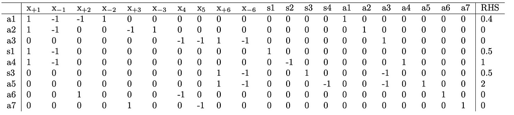
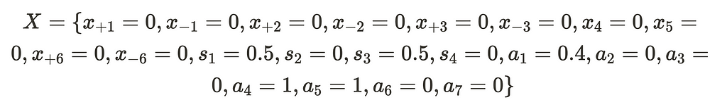
To identify a feasible point, the simplex method initially checks if setting all slack variables to the right-hand side and all other variables to zero is feasible. In our case, this approach is not viable due to non-zero equality constraints lacking a slack variable. Additionally, on lines 5 and 7, the slack variable is multiplied by a negative number, making it impossible for the expression to evaluate to positive right-hand sides, as slack variables are always positive. Therefore, to obtain an initial feasible point, we will introduce new auxiliary variables assigned to be equal to the right-hand side, setting all other variables to zero. This won’t be done for constraints with positive signed slack variables, as those slack variables may already equal the right-hand side. To enhance clarity, we will add a column on the left indicating which variables are assigned a non-zero value; these are referred to as our basic variables.
Our feasible point then is
It’s important to recognize that these auxiliary variables alter the solution, and in order to arrive at our desired true solution we need to eliminate them. To eliminate them, we will introduce an objective function to set them to zero. Specifically, we aim to minimize the function. a1 + a2 + a3 + a4 + a5 + a6 + a7. If we successfully minimize this function to zero, we can conclude that our original set of equations has a feasible point. However, if we are unable to achieve this, it indicates that there is no feasible point, allowing us to terminate the problem.
With the tableau and objective function declared, we are prepared to execute the pivots necessary to optimize our objective. The steps for doing which are as follows:
- Replace basic variables in objective function with non-basic variables. In this case, all the auxiliary variables are basic variables. To replace them, we pivot on all of the auxiliary columns and the rows that have a non-zero value entry for the basic variable. A pivot is done by adding or subtracting from the pivot row to all other rows until the only non-zero entry in the pivot column is the entry in the pivot row.
- Select a pivot column by finding the column with the first and largest value in the objective function.
- Select a pivot row by using bland’s rule. Bland’s rule we identify all positive entries in our column, divide the objective by those entries, and choose the row that yields the smallest value.
- Repeat steps 2 and 3 until all entries in the objective function are non-positive.
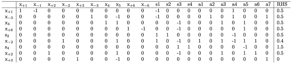
Once this done, we will have the following new tableau.
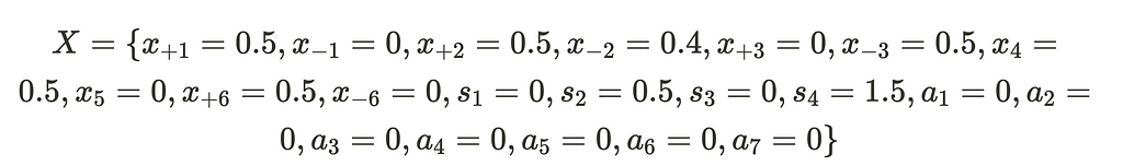
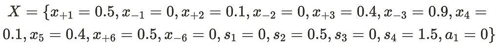
From this, we arrive at the point
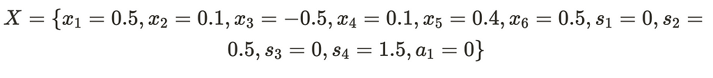
We have successfully adjusted all of the auxiliary variables to equal zero. We also have pivoted away from them to make them all non-basic. Also, we will note that these values do indeed satisfy our initial linear constraints. As such, we no longer need the auxiliary variables may remove them from our set of linear equations. If we collapse the positive and negative variables and remove the auxilary variables we have this new point:
Relu Fix Search Procedure
By adding the constraints x_{+2} = x_4 and x_{+3} = x_5 we make it possible for both x_{+2} and x_{-2} to both be non-zero (same applies for x_{+3} and x_{-3} ). As can be seen above, both x_{+2} and x_{-2} are non-zero and relu(x_2) does not equal x_4. To fix the ReLU, there is no way to directly constrain simplex to either have x_{+2} or x_{-2} be zero, we must choose one case and create a constraint for that case. Choosing between these two cases is equivalent to deciding whether the ReLU will be in an active or inactive state. In the original paper, the authors address ReLU violations by assigning one side to equal the value of the other side at that specific moment. We believe this approach overly constrains the problem. That is because limiting the ReLU to a specific value and necessitating potentially an infinite number of configurations to check. Our solution, on the other hand, constrains the ReLU to be either active or inactive. Consequently, we only need to check these situations to cover the space of all allowable configurations.
As we need to decide whether the ReLU constraints are active or inactive, and with 2 to the n valid constraints to set, manually examining all possible configurations in a large network becomes impractical.
The authors of Reluplex propose addressing violations by attempting to solve them one ReLU fix at a time. They iteratively add one constraint to fix one specific violation, update the tableau to accomodate the new constraint, remove the constraint, then repeat for all other or new violations. Because only one constraint is ever in place it is possible that updating one ReLU fix can break one in another place that was already fixed. This can lead to a cycle of repeatedly fixing the same ReLU constraints. To get around this, if a ReLU node is updated five times, a “ReLU split” is executed. This split divides the problem into two cases: in one, they enforce that the negative side of the variable is zero, and in the other, the positive side is set to zero. Importantly, the constraint is not removed in either case, ensuring that the particular ReLU will never need fixing again. This allows the algorithm to only split on particularly “problematic” ReLU nodes, and empirical evidence shows that typically only about 10% of ReLUs need to split. Consequently, although some fixing operations may be repeated, the overall procedure remains faster than a simple brute-force check for every possibility.
Adding Constraint To Fix Relu
To address the ReLU violation, we need to constrain either x_{+2} or x_{-2} to be zero. To maintain a systematic approach, we will consistently attempt to set the positive variable to zero first. If that proves infeasible, we will then set the negative side to zero.
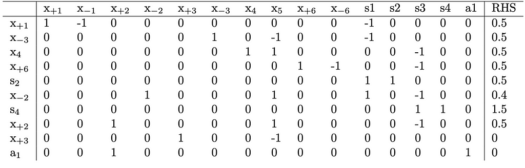
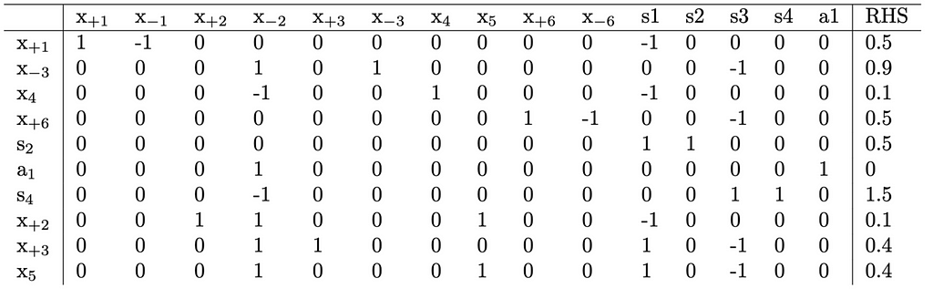
Introducing a new constraint involves adding a new auxiliary variable. If we add this variable and impose a constraint to set x_{+2}=0, the tableau is transformed as follows:
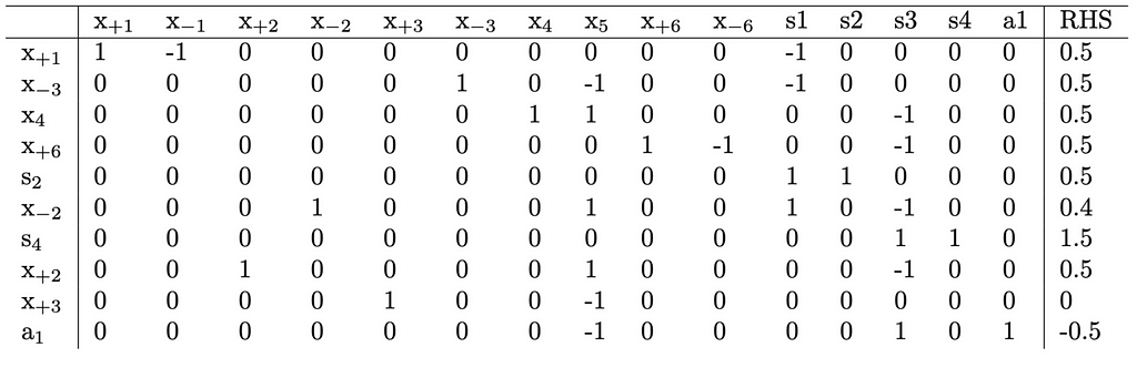
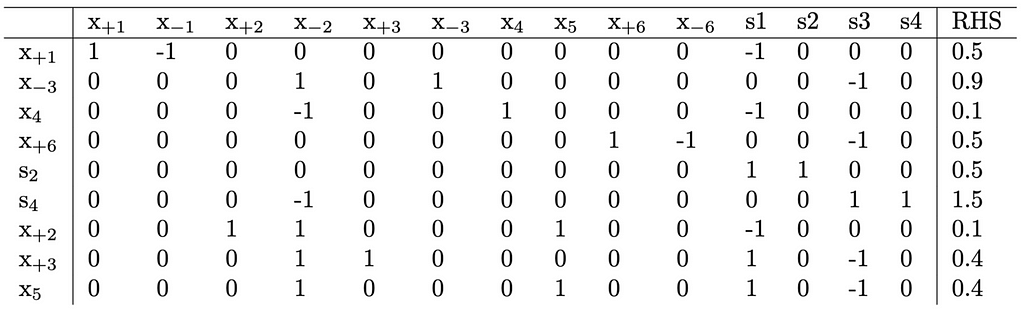
x_{+2} functions as a basic variable and appears in two distinct rows. This contradicts one of the assumptions necessary for the simplex method to function properly. Consequently, a quick pivot on (x_{+2}, x_{+2}) is necessary to rectify this issue. Executing this pivot yields the following:
Solving The Dual Problem
In the previous step, we applied the two-phase method to solve the last tableau. This method involves introducing artificial variables until a guaranteed trivial initial point is established. Subsequently, it pivots from one feasible point to another until an optimal solution is attained. However, instead of continuing with the two-phase method for this tableau, we will employ the dual simplex method.
The dual simplex method initiates by identifying a point that is optimally positioned beyond the given constraints, often referred to as a super-optimal point. It then progresses from one super-optimal point to another until it reaches a feasible point. Once a feasible point is reached, it is ensured to be the global optimal point. This method suits our current scenario as it enables us to add a constraint to our already solved tableau without the need to solve a primal problem. Given that we lack an inherent objective function, we will assign an objective function as follows:
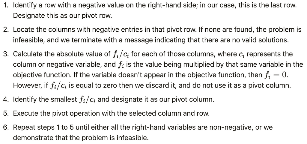
Solving the Primal Problem typically involves transposing the matrix and replacing the objective function values with the right-hand side values. However, in this case, we can directly solve it using the tableau we’ve already set up. The process is as follows:
Applying this procedure to the problem we’ve established will reveal its infeasibility. This aligns with expectations since setting x_{+3} to zero would necessitate setting x_{+1}-x_{-1} or x_1 to 0.4 or lower, falling below the lower bound constraint of 0.5 we initially imposed on x_1.
Setting x_{-1}=0
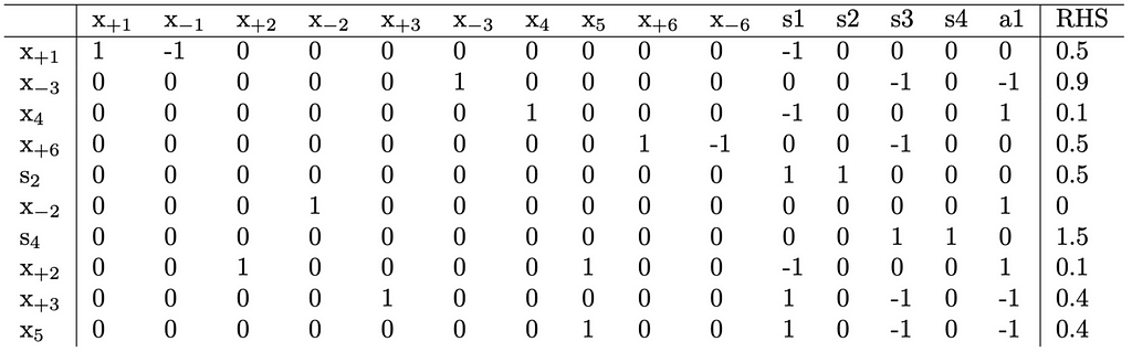
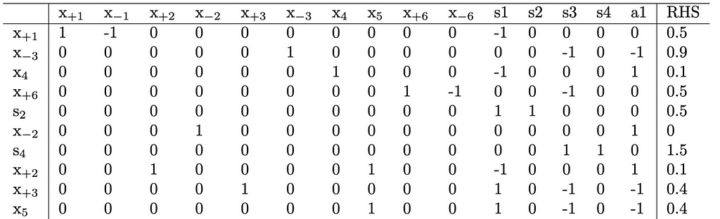
Since setting x_{+1}=0 failed, we move on to trying to set x_{-1}=0. This actually will succeed and result in the following completed tableau:
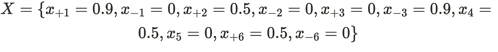
From this, we have the new solution point:
Which if we collapse becomes:
Now that we have successfully made x_4 = relu(x_2) , we must remove the temporary constraint before we continuing.
Removing The Temporary ReLU Constraint
To lift the constraint, a pivot operation is required to explicitly state the constraint within a single row. This can be achieved by pivoting on our new a_1 column. Following Bland’s rule for selecting the pivot row, we identify all positive entries in our column, divide the objective by those entries, and choose the row that yields the smallest value. In this instance, the x_{-2} row emerges as the optimal choice since 0/1=0 is smaller than all other candidates. After performing the pivot, the resulting tableau is as follows:
It’s important to observe that none of the variable values have been altered. We can now confidently eliminate both the a_1 row and a_1 column from the tableau. This action effectively removes the constraint x_{-2}=0, resulting in the following updated tableau:
Continuing to Relu Split
As evident, we successfully addressed the ReLU violation, achieving the desired outcome of x_4 = ReLU(x_2). However, a new violation arises as x_5 does not equal ReLU(x_3). To fix this new violation, we follow the exact same procedure we used to fix the x_4 does not equal ReLU(x_2) violation. Once this is done though, we find that the tableau reverts to its state before we fixed x_4 = ReLU(x_2). If we continue, we will cycle between fixing x_4 = ReLU(x_2) and x_5 = ReLU(x_3) until we have updated one of these enough for a ReLU split to be triggered. This split creates two tableaus: one where x_{+2}=0 (shown to be infeasible) and another where x_{-2}=0, resulting in a tableau we have encountered before.
This time though, we will proceed without removing the constraint x_{-2}=0. Trying to fix the x_{+3}=0 constraint will be successful and result in the following values:
Which when we collapse becomes:
This outcome is free of ReLU violations and represents a valid point that the neural network can produce within the initially declared bounds. With this, our search concludes, and we can officially declare it complete.
Possible Optimizations
A significant optimization opportunity lies in cases where only one side of the ReLU is feasible. In such instances, it is unnecessary to remove the constraint. This is because, in those scenarios, we are not imposing any additional constraints, allowing us to conclude that if a side is infeasible, it will remain so indefinitely, regardless of additional constraints. Therefore, there is no need to remove the constraint on the feasible side. In our toy example, this optimization would have reduced the required updates from 13 to only 3. However, it’s important to note that we shouldn’t necessarily expect a proportionate improvement in larger networks. This optimization is used in our python implementation.
The original paper suggests other optimizations such as bound tightening, derived bounds, conflict analysis, and floating-point arithmetic. However, these optimizations are not implemented in our solution.
Code Implementations
For the best-performing and production-ready version of the algorithm, we suggest exploring the official Marabou GitHub page[5]. Additionally, you can delve into the official Reluplex repository for a more in-depth understanding of the algorithm[2]. The author has written a simplified implementation of ReLuPlex in Python[3]. This implementation can be valuable for grasping the algorithm and can serve as a foundation for developing a customized Python version of the algorithm.
References
[1][1702.01135] Reluplex: An Efficient SMT Solver for Verifying Deep Neural Networks (arxiv.org)
[2][1803.08375] Deep Learning using Rectified Linear Units (ReLU)
[2] Official Implementation of ReluPlex (github.com)
[3] Python Implementation of ReluPlex by author (github.com)
[4][1910.14574] An Abstraction-Based Framework for Neural Network Verification (arxiv.org)
[5] Official Implementation Of Marabou (github.com)
[6][2210.13915]Towards Formal XAI: Formally Approximate Minimal Explanations of Neural Networks
[7] Neural Networks By Science Direct
[8]Comprehensive Overview of Backpropagation Algorithm for Digital Image Denoising
Implementation Details Of Reluplex: An Efficient SMT Solver for Verifying Deep Neural Networks was originally published in Towards Data Science on Medium, where people are continuing the conversation by highlighting and responding to this story.
Denial of responsibility! Techno Blender is an automatic aggregator of the all world’s media. In each content, the hyperlink to the primary source is specified. All trademarks belong to their rightful owners, all materials to their authors. If you are the owner of the content and do not want us to publish your materials, please contact us by email – [email protected]. The content will be deleted within 24 hours.