Implementing, solving and visualizing the Traveling Salesman Problem with Python

Implementing, Solving, and Visualizing the Traveling Salesman Problem with Python

Translate an optimization model from math to Python, optimize it, and visualize the solution to gain quick feedback on modeling errors

👁️ This is article #3 of the series covering the project “An Intelligent Decision Support System for Tourism in Python”. I encourage you to check it out to get a general overview of the whole project. If you’re only interested in how to implement a model of the TSP in Python, you’re still at the right place: this article is self-contained, and I will walk you through all the steps—installation of dependencies, analysis, code, interpretation of results, and model debugging.

The present article continues our journey right where sprint 2 left off. Here, we take the mathematical model we formulated in the previous article, and implement it in Python, using Pyomo, and following good practices. Then, the model is optimized, and its solutions are visualized and analyzed. For pedagogy’s sake, we find that the initial model formulation is incomplete, so I show how we can derive, from first principles, the constraints needed to fix the formulation. These new constraints are added to the Pyomo model, and the new solutions are analyzed again and verified.

Table of contents

1. Implementing the model in Python using Pyomo

• 1.1. Installing the dependencies
• 1.2. Math becomes code

2. Solving and validating the model

• 2.1. Solving the model
• 2.2. Visualizing the results
• 2.3. Analyzing the results

3. Fixing the formulation

• 3.1. The motivating idea
• 3.2. Expressing the motivating idea as logical implications
• 3.3. Formulating the logical implications as linear constraints
• 3.4. Deducing a proper value for the “big M”

4. Implementing and verifying the new formulation

• 4.1. Augmenting the Pyomo model
• 4.2. Plotting the updated model’s solution

5. Conclusion (for next sprint)

📖 If you didn’t read the previous article, worry not. The mathematical formulation is also stated (but not derived) here, with each model component next to its code implementation. If you don’t understand where things come from or mean, please read the article of “sprint 2”, and if you’d like more context, read the article for “sprint 1".

1. Implementing the model in Python using Pyomo

Python is used as it’s the top language in data science, and Pyomo as it’s one of the best (open-source) libraries that deal effectively with large-scale models.

In this section, I’ll go through each model component defined in the formulation, and explain how it is translated to Pyomo code. I’ve tried to not leave any gaps, but if you feel otherwise, please leave a question in the comments.

Disclaimer: The target reader is expected to be new to Pyomo, and even to modeling, so to lower their cognitive burden, concise and simple implementation is prioritized over programming best practices. The goal now is to teach optimization modeling, not software engineering. The code is incrementally improved in future iterations as this proof-of-concept evolves into a more sophisticated MVP.

1.1. Installing the dependencies

For people in a hurry

Install (or make sure you already have installed) the libraries pyomo, networkx and pandas, and the package glpk.

📝 The package glpk contains the GLPK solver, which is an (open source) external solver we will use to optimize the models we create. Pyomo is used to create models of problems and pass them to GLPK, which will run the algorithms that carry out the optimization process itself. GLPK then returns the solutions to the Pyomo model object, which are stored as model attributes, so we can use them conveniently without leaving Python.

The recommended way to install GLPK is through conda so that Pyomo can find the GLPK solver easily. To install all dependencies together in one go, run:

conda install -y -c conda-forge pyomo=6.5.0 pandas networkx glpk

For organized people

I recommend creating a separate virtual environment in which to install all the libraries needed to follow the articles in this series. Copy this text

name: ttp  # traveling tourist problem
channels:
  - conda-forge
dependencies:
  - python=3.9
  - pyomo=6.5.0
  - pandas
  - networkx
  - glpk  # external solver used to optimize models
  - jupyterlab  # comment this line if you won't use Jupyter Lab as IDE

and save it in a YAML file named environment.yml. Open an Anaconda prompt in the same location and run the command

conda env create --file environment.yml

After some minutes, the environment is created with all the dependencies installed inside. Run conda activate ttp to "get inside" the environment, fire up Jupyter Lab (by running jupyter lab in the terminal), and start coding along!

1.2. Math becomes code

First, let’s make sure the GLPK solver is findable by Pyomo

### =====  Code block 3.1  ===== ###
import pandas as pd
import pyomo.environ as pyo
import pyomo.version
import networkx as nx


solver = pyo.SolverFactory("glpk")
solver_available = solver.available(exception_flag=False)
print(f"Solver '{solver.name}' available: {solver_available}")

if solver_available:
    print(f"Solver version: {solver.version()}")

print("pyomo version:", pyomo.version.__version__)
print("networkx version:", nx.__version__)

Solver 'glpk' available: True
Solver version: (5, 0, 0, 0)
pyomo version: 6.5
networkx version: 2.8.4

⛔ If you got the message 'glpk' available: False, the solver didn't install properly. Please try one of these to fix the issue:

– re-do the installation steps carefully

– run conda install -y -c conda-forge glpk in the base (default) environment

– try to install a different solver that works for you

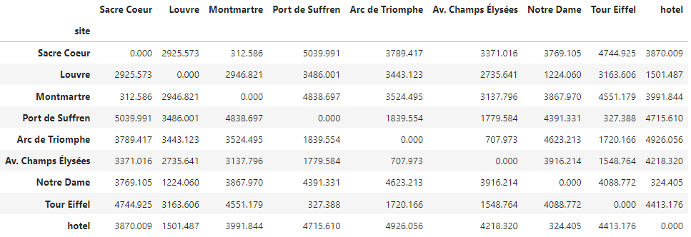
Then read the distance data CSV file

### =====  Code block 3.2  ===== ###
path_data = (
    "https://raw.githubusercontent.com/carlosjuribe/"
    "traveling-tourist-problem/main/"
    "Paris_sites_spherical_distance_matrix.csv"
)
df_distances = pd.read_csv(path_data, index_col="site")

df_distances

Now we enter “stage 4” of the [Agile Operations Research workflow], marked as the green block below:

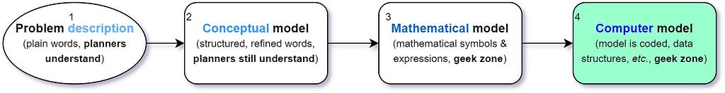
The task is to take the mathematical model created earlier and implement it in code exactly as it was defined mathematically.

👁️ We are allowed to create as many Python objects as we want if that makes the model implementation easier, but we are not allowed to modify the underlying model in any way, while we’re coding it. It would cause the math model and the computer model to be out-of-sync, thereby making later model debugging pretty hard.

We instantiate an empty Pyomo model, in which we will store model components as attributes:

model = pyo.ConcreteModel("TSP")

1.2.1. Sets

In order to create the set of sites 𝕊 = {Louvre, Tour Eiffel, …, hotel}, we extract their names from the index of the dataframe and use it to create a Pyomo Set named sites:

### =====  Code block 3.3  ===== ###
list_of_sites = df_distances.index.tolist()

model.sites = pyo.Set(initialize=list_of_sites, 
                      domain=pyo.Any, 
                      doc="set of all sites to be visited (𝕊)")

To create the derived set

We store the filter 𝑖 ≠ 𝑗 inside a construction rule (the Python function _rule_domain_arcs), and pass this rule to the filter keyword when initializing the Set. Note that this filter will be applied to the cross-product of the sites (𝕊 × 𝕊), and will filter out those members of the cross-product that do not satisfy the rule.

### =====  Code block 3.4  ===== ###
def _rule_domain_arcs(model, i, j):
    """ All possible arcs connecting the sites (𝔸) """
    # only create pair (i, j) if site i and site j are different
    return (i, j) if i != j else None 

rule = _rule_domain_arcs
model.valid_arcs = pyo.Set(
    initialize=model.sites * model.sites,  # 𝕊 × 𝕊
    filter=rule, doc=rule.__doc__)

1.2.2. Parameters

The parameter

𝐷ᵢⱼ ≔ Distance between site 𝑖 and site 𝑗

is created with the constructor pyo.Param, which takes as the first (positional) argument the domain 𝔸 (model.valid_arcs) that indexes it, and as the keyword argument initialize another construction rule, _rule_distance_between_sites, that is evaluated for each pair (𝑖, 𝑗) ∈ 𝔸. In each evaluation, the numeric value of the distance is fetched from the dataframe df_distances, and linked internally to the pair (𝑖, 𝑗):

### =====  Code block 3.5  ===== ###
def _rule_distance_between_sites(model, i, j):
    """ Distance between site i and site j (𝐷𝑖𝑗) """
    return df_distances.at[i, j]  # fetch the distance from dataframe

rule = _rule_distance_between_sites
model.distance_ij = pyo.Param(model.valid_arcs, 
                              initialize=rule, 
                              doc=rule.__doc__)

1.2.3. Decision variables

Because 𝛿ᵢⱼ has the same “index domain” as 𝐷ᵢⱼ, the way to build this component is very similar, with the exception that no construction rule is needed here.

model.delta_ij = pyo.Var(model.valid_arcs, within=pyo.Binary, 
                         doc="Whether to go from site i to site j (𝛿𝑖𝑗)")

The first positional argument of pyo.Var is reserved for its index set 𝔸, and the "type" of variable is specified with the keyword argument within. With "type of variable" I mean the range of values that the variable can take. Here, the range of 𝛿ᵢⱼ is just 0 and 1, so it is of type binary. Mathematically, we would write 𝛿ᵢⱼ ∈ {0, 1}, but instead of creating separate constraints to indicate this, we can indicate it directly in Pyomo by setting within=pyo.Binary at the time we create the variable.

1.2.4. Objective function

To construct an objective function we can “store” the expression in a function that will be used as the construction rule for the objective. This function only takes one argument, the model, which is used to fetch any model component needed to build the expression.

### =====  Code block 3.6  ===== ###
def _rule_total_distance_traveled(model):
    """ total distance traveled """
    return pyo.summation(model.distance_ij, model.delta_ij)

rule = _rule_total_distance_traveled
model.obj_total_distance = pyo.Objective(rule=rule, 
                                         sense=pyo.minimize, 
                                         doc=rule.__doc__)

Observe the parallelism between the mathematical expression and the return statement of the function. We specify that this is a minimization problem with the sense keyword.

1.2.5. Constraints

If you recall from the previous article, a convenient way to enforce that each site is visited only once is by enforcing that each site is “entered” once and “exited” once, simultaneously.

Each site is entered just once

def _rule_site_is_entered_once(model, j):
    """ each site j must be visited from exactly one other site """
    return sum(model.delta_ij[i, j] for i in model.sites if i != j) == 1

rule = _rule_site_is_entered_once
model.constr_each_site_is_entered_once = pyo.Constraint(
                                          model.sites, 
                                          rule=rule, 
                                          doc=rule.__doc__)

Each site is exited just once

def _rule_site_is_exited_once(model, i):
    """ each site i must departure to exactly one other site """
    return sum(model.delta_ij[i, j] for j in model.sites if j != i) == 1

rule = _rule_site_is_exited_once
model.constr_each_site_is_exited_once = pyo.Constraint(
                                          model.sites, 
                                          rule=rule, 
                                          doc=rule.__doc__)

1.2.6. Final inspection of the model

The model implementation is done. To see what it looks like as a whole, we should execute model.pprint(), and navigate a bit around to see if we missed some declarations or made some mistakes.

To get an idea of the size of the model, we print the number of variables and constraints that it is made of:

def print_model_info(model):
    print(f"Name: {model.name}", 
          f"Num variables: {model.nvariables()}",
          f"Num constraints: {model.nconstraints()}", sep="\n- ")

print_model_info(model)

#[Out]:
# Name: TSP
#  - Num variables: 72
#  - Num constraints: 18

Having fewer than 100 constraints or variables, this is a small-size problem, and it will be optimized relatively fast by the solver.

2. Solving and validating the model

2.1. Solving the model

The next step in the [AOR flowchart] is to optimize the model, and inspect the solutions:

res = solver.solve(model)  # optimize the model
print(f"Optimal solution found: {pyo.check_optimal_termination(res)}")
# [Out]: Optimal solution found: True

Good news! The solver has found an optimal solution to this problem! Let’s check it so that we can know what tour to follow when we get to Paris!

For a very quick check, we can run model.delta_ij.pprint(), which will print all the (optimal) values of the 𝛿ᵢⱼ variables, being either 0 or 1:

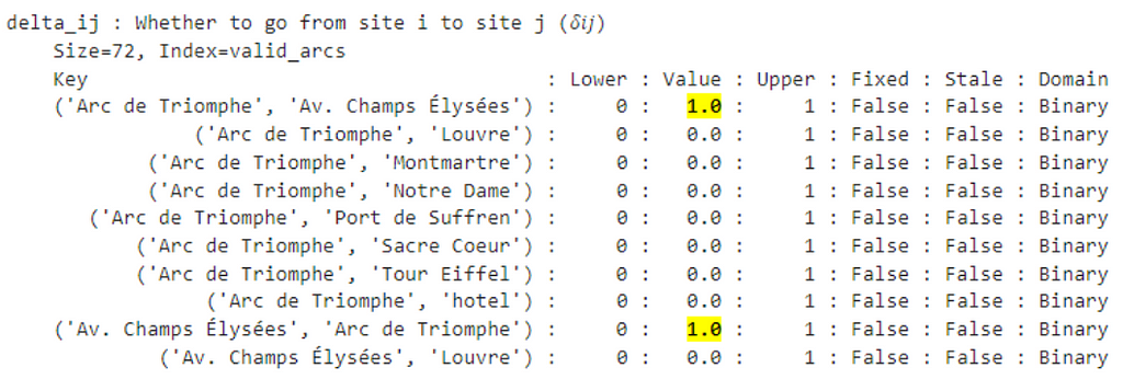
It’s difficult to visualize a tour merely by looking at a list of chosen arcs, let alone analyze it to validate that we formulated the model correctly.

To really understand the solution, we need to visualize it.

2.2. Visualizing the results

An image is worth a thousand records

As we’re dealing with nodes and arcs, the easiest way to visualize the solution is to plot it as a graph. Remember that this is a proof-of-concept, so quick, effective feedback trumps beauty. The more insightful visualizations can wait until we have a working MVP. For now, let’s write some helper functions to plot solutions efficiently. The

The function extract_solution_as_arcs takes in a solved Pyomo model and extracts the "chosen arcs" from the solution. Next, the function plot_arcs_as_graph stores the list of active arcs in a Graph object for easier analysis and plots that graph so that the hotel is the only red node, for reference. Lastly, the function plot_solution_as_graph calls the above two functions to display the solution of the given model as a graph.

### =====  Code block 3.7  ===== ###
def extract_solution_as_arcs(model):
    """ Extract list of active (selected) arcs from the solved model,
    by keeping only the arcs whose binary variables are 1 """
    active_arcs = [(i, j)
                   for i, j in model.valid_arcs
                   if model.delta_ij[i, j].value == 1]
    return active_arcs


def plot_arcs_as_graph(tour_as_arcs):
    """ Take in a list of tuples representing arcs, convert it 
    to a networkx graph and draw it
    """
    G = nx.DiGraph()
    G.add_edges_from(tour_as_arcs)  # store solution as graph

    node_colors = ['red' if node == 'hotel' else 'skyblue' 
                   for node in G.nodes()]
    nx.draw(G, node_color=node_colors, with_labels=True, font_size=6, 
            node_shape='o', arrowsize=5, style='solid')

    
def plot_solution_as_graph(model):
    """ Plot the solution of the given model as a graph """
    print(f"Total distance: {model.obj_total_distance()}")
    
    active_arcs = extract_solution_as_arcs(model)
    plot_arcs_as_graph(active_arcs)

Now we can see what the solution really looks like:

plot_solution_as_graph(model)

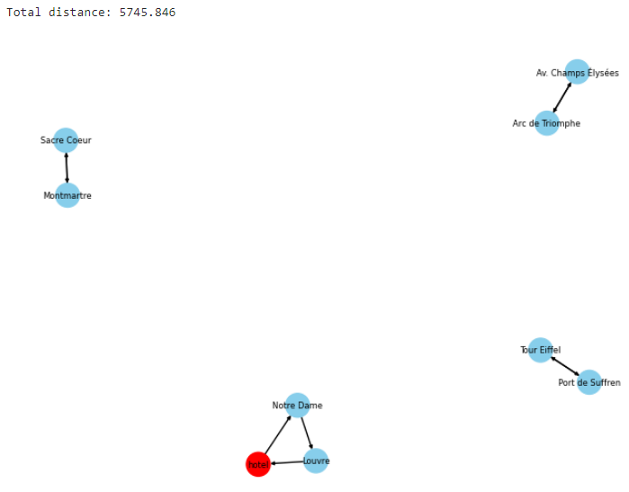
Well, this is obviously not what we expected! There is no single tour traversing all sites and coming back to the hotel. It’s true that all sites are visited, but only as part of small disconnected clusters of sites. Technically, yes, the constraints we specified are carefully obeyed: each site is entered just once and exited just once, but the overall result is not one single tour, as we intended, but a group of subtours. This means that the assumption we did in the previous article is wrong, so something else is missing in the model that will encode the requirement that “subtours are not permitted in the solution”.

2.3. Analyzing the results

What has gone wrong?

When the solution of a model does not make sense, there’s only one possible explanation: the model is wrong¹.

The solver gave us what truly is the optimal solution to the model, but we gave it a model that does not map to the problem we want to solve. The task is now to find out why, and where we made a mistake. On reflection, the obvious candidate is the dubious assumption we made in the last two paragraphs of section “4.4. Creating the constraints” in the predecessor article, where we designed the mathematical model. We (wrongly, as we now know) assumed that the formation of a single tour would follow naturally from the two constraints that ensure each site is visited just once. But as we just visualized, it doesn’t. Why?

The root cause of the error lies in what I call “unspoken common-sense”: knowledge we have about the world that is so obvious that we forget to specify it in a model

We knew, implicitly, that teleportation is not possible when visiting sites, but we didn’t explicitly tell the model. That’s why we observe those little subtours, connecting some of the sites, but not all. The model “thinks” it’s okay to teleport from one site to another, as long as, once it’s on a site, it is exited once and entered once (see Figure 3.2 again). If we see subtours is only because we told the model to minimize the tour’s distance, and just so happens that teleportation is helpful at saving distance.

Thus, we need to prevent the formation of these subtours to obtain a realistic solution. We need to design some new constraints that “tell the model” that subtours are forbidden, or, equivalently, that the solution must be a single tour. Let’s go with the latter, and deduce, from first principles, one set of constraints that is intuitive and does the job fine.

3. Fixing the formulation

Referring to the [Agile Operations Research workflow], we are now in the model reformulation phase. A reformulation of a model could be about improving it or fixing it. Ours will be about fixing it.

We know what we want: to force the solution to be a single tour, starting and ending at our initial site, the hotel. The challenge is how to encode that requirement into a set of linear constraints. Below is one idea, stemming from the properties of a tour.

3.1. The motivating idea

We have 𝑁 sites to “traverse”, including the hotel. Since we start at the hotel, that means 𝑁 − 1 sites left to visit. If we keep track of the “chronological order” in which we visit those sites, such that the first destination (after the hotel) is given the number 1, the second destination is given the number 2, and so on, then the last destination before returning to the hotel will be given the number 𝑁 − 1. If we call these numbers used to track the order of visits “ranks”, then the pattern that occurs in the tour is that the rank of any site (other than the hotel) is always 1 unit higher than the rank of the site that preceded it in the tour. If we could formulate a set of constraints that impose such a pattern on any feasible solution, we would be, loosely speaking, introducing a “chronological order” requirement in the model. And it turns out we can indeed.

3.2. Expressing the motivating idea as logical implications

💡 This is the “pattern” that we want any feasible solution to satisfy:

The rank of any site (other than the hotel) must always be 1 unit higher than the rank of the site that preceded it in the tour

We can re-express this pattern as a logical implication, like this: “the rank of site 𝑗 must be 1 unit higher than the rank of site 𝑖 if and only if 𝑗 is visited right after 𝑖, for all arcs (𝑖, 𝑗) that do not include the hotel 𝐻”. This wording is expressed mathematically as:

where 𝑟ᵢ are the new variables we need to keep track of the (yet unknown) order of visits. To distinguish them from the decision variables, let’s call them “rank variables”. The right side is read as “for all 𝑖 and 𝑗 belonging to the set of all sites excluding the hotel”. For notational convenience, we define the new set 𝕊* to store all the sites except the hotel (denoted by 𝐻):

which allows us to define the rank variables concisely as:

👁️ It’s crucial that the hotel does not have an associated rank variable because it will be simultaneously the origin and final destination of any tour, a condition that would violate the pattern of “ever increasing rank variables in the tour”. This way, the rank of each site is always forced to increase with any new arc taken, which ensures that closed loops are prohibited unless the loops close at the only site that doesn’t have a rank variable: the hotel

The bounds of 𝑟ᵢ are derived from its description: the rank starts at 1 and monotonically increases until all sites in 𝕊* are visited, thus ending at | 𝕊* | (the size of the set of non-hotel sites). Besides, we allow them to take any positive real value:

3.3. Formulating the logical implications as linear constraints

The challenge now is to translate this logical implication to a set of linear constraints. Thankfully, linear inequalities serve also the purpose of enforcing logical implications, not just finite resource limitations.

One way to do that is through the so-called Big-M method, which consists of declaring a constraint in such a way that, when the condition you care about is met, the constraint applies (becomes active), and when the condition you care about is not met, the constraint becomes redundant (becomes inactive). The technique is called “big-M” because it makes use of a constant value 𝑀 that is sufficiently large so as to, when appearing in the constraint, render it redundant for every case. When 𝑀 does not appear in the constraint, the constraint is “active” in the sense that it is enforcing the desired implication.

But what determines whether a constraint is “active” or not? The short answer is the values of the decision variables themselves that the constraint applies to. Let’s see how it works.

The desired implication is to have 𝑟ⱼ = 𝑟ᵢ + 1 only when 𝛿ᵢⱼ = 1. We can replace the 1 in the expression with 𝛿ᵢⱼ, which yields

This is the relation we want to hold when 𝛿ᵢⱼ = 1, but not when 𝛿ᵢⱼ = 0. To “correct” for the case when 𝛿ᵢⱼ = 0, we add a redundancy term, 𝑅𝑇, whose function is to “deactivate the constraint” only when 𝛿ᵢⱼ = 0. Therefore, this redundancy term must include the variable 𝛿ᵢⱼ, as it depends on it.

In this context, “deactivating the constraint” stands for “making it redundant”, since a redundant constraint has the same effect as a non-existing constraint in a model.

Let’s see how we can deduce the expression for RT. The expression for 𝑅𝑇(𝛿ᵢⱼ) needs to satisfy these properties:

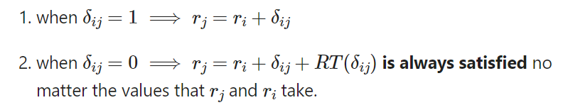
To satisfy point (1) we need 𝑅𝑇(𝛿ᵢⱼ = 1) = 0, and thus the expression for 𝑅𝑇 must contain the multiplier (1 − 𝛿ᵢⱼ), as it becomes 0 when 𝛿ᵢⱼ =1. This form makes 𝑅𝑇 “vanish” when 𝛿ᵢⱼ = 1, or “be reduced” to a constant (let’s call it M) when 𝛿ᵢⱼ = 0. Thus, a candidate for the redundancy term is

where 𝑀 should be determined from the problem data (more on that later).

To satisfy point (2) for all possible 𝑖’s and 𝑗’s, we need to make the equality in expression (3.11) an inequality (= becomes ≥), and find a constant 𝑀 big enough (in absolute value) so that, no matter what values 𝑟ⱼ and 𝑟ᵢ take, the constraint is always satisfied. This is where the “big” in “big M” comes from.

Once we find such a sufficiently large constant 𝑀, our “logical implication” constraint will take the form

Introducing these constraints into the model will, presumably, force the solution to be a single tour. But the constraints won’t have the desired effect unless we first specify a good value for M.

3.4. Deducing a proper value for the “big M”

Since the goal is to have 𝑅𝑇(𝛿ᵢⱼ = 0) = 𝑀, we can deduce a proper value for 𝑀 by setting 𝛿ᵢⱼ = 0 in the general constraint stated in Expression (3.12):

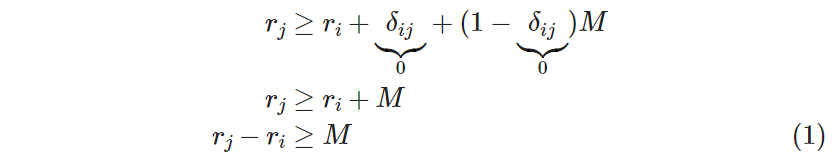
For 𝑟ⱼ − 𝑟ᵢ ≥ 𝑀 to be satisfied for all non-hotel sites 𝑖, 𝑗, we need the lower bound of 𝑟ⱼ − 𝑟ᵢ to be also greater than 𝑀. The lower bound (LB) of 𝑟ⱼ − 𝑟ᵢ is the minimum value that 𝑟ⱼ − 𝑟ᵢ can take, and can be obtained by

where 𝑟ᵐⁱⁿ is the minimum possible rank and 𝑟ᵐᵃˣ the maximum possible rank. Therefore, for inequality (1) in Expression (3.13) to be true for all ranks of all sites, the following inequality must hold too:

Thanks to this inequality we know the minimum value that 𝑀 must take in order for the big-M method to work, which is

And what are the values of 𝑟ᵐⁱⁿ and 𝑟ᵐᵃˣ? In our convention, we gave the first visited site the rank 1, which is, of course, the minimum rank (i.e., 𝑟ᵐⁱⁿ = 1). Since the rank grows by 1 unit in each site visited, the last non-hotel site in the tour will have the maximum rank, equal to the number of all non-hotel sites. As the number of non-hotel sites can vary, we need a general expression. If you remember, we defined the set 𝕊* to contain all non-hotel sites, so the number we’re after is the size (i.e., the number of elements) of the set 𝕊*, which in math notation is expressed as | 𝕊* |. Thus, we have deduced that 𝑟ᵐⁱⁿ = 1 and 𝑟ᵐᵃˣ = | 𝕊* |. Substituting in Expression (3.14), we finally arrive at a proper value for M:

Because 𝕊* will always have more than 2 sites to be visited (otherwise, there would be no decision problem at all in the first place), the “big M” value, in this model, is always a negative “big” value”.

📝 Theoretical values versus computational values

Theoretically, we are allowed to choose arbitrarily “more negative” values for 𝑀 than the one deduced here—even make up huge numbers to be sure they’re big enough, to avoid this calculation — but this is not good practice. If 𝑀 gets too large (in absolute value), it can create performance issues in the solver’s algorithms, or, in the worst case scenario, even make the solver consider infeasible solutions as feasible. That’s why the recommended practice is to derive, from the problem’s data, a tight, but sufficiently large value for 𝑀.

Now that we have deduced a proper value for “big M”, we will store it in a new model parameter, for easier reuse. With this, the subtour elimination constraint set is ready, and its “full form” is

To keep things in perspective, note that this is actually the “constraint equivalent” of the original logical implication we formulated earlier in Expression (3.6):

Congratulations! We finally have a set of constraints that can be added to our model. Coming up with them was the hard part. Now, let’s verify that their addition to the model really results in the disappearance of subtours.

4. Implementing and verifying the new formulation

4.1. Augmenting the Pyomo model with the new formulation

Revising and correcting the model has required the addition of a few more sets, parameters, variables, and constraints. Let’s add these new model components to the Pyomo model, following the same order as in the initial formulation phase.

4.1.1. Sets and parameters

• Sites of interest, 𝕊*: set of all sites excluding the hotel:

Pyomo Set objects have operations compatible with Python sets, so we can do the difference between a Pyomo set and a Python set directly:

model.sites_except_hotel = pyo.Set(
    initialize=model.sites - {'hotel'}, 
    domain=model.sites,
    doc="Sites of interest, i.e., all sites except the hotel (𝕊*)"
)

• big M, the new parameter for the subtour elimination constraint:

model.M = pyo.Param(initialize=1 - len(model.sites_except_hotel),
                    doc="big M to make some constraints redundant")

4.1.2. Auxiliary variables

• rank variables, rᵢ: to keep track of the order in which sites are visited:

model.rank_i = pyo.Var(
    model.sites_except_hotel,  # i ∈ 𝕊* (index)
    within=pyo.NonNegativeReals,  # rᵢ ∈ ℝ₊ (domain)
    bounds=(1, len(model.sites_except_hotel)),  # 1 ≤ rᵢ ≤ |𝕊*|
    doc="Rank of each site to track visit order"
)

In the comments, you can see how nicely the elements of the full mathematical definition of the variables map to the arguments of the Pyomo variable declaration function pyo.Var. I hope this helps you appreciate the value of having a well-defined mathematical model before starting to build a Pyomo model. The implementation will just flow naturally, and errors will be less likely.

4.1.3. Constraints

• The solution must be a single tour starting and ending at the hotel:

def _rule_path_is_single_tour(model, i, j):
    """ For each pair of non-hotel sites (i, j), 
    if site j is visited from site i, the rank of j must be 
    strictly greater than the rank of i. """
    if i == j:  # if sites coincide, skip creating a constraint
        return pyo.Constraint.Skip
    
    r_i = model.rank_i[i]
    r_j = model.rank_i[j]
    delta_ij = model.delta_ij[i, j]
    return r_j >= r_i + delta_ij + (1 - delta_ij) * model.M

# cross product of non-hotel sites, to index the constraint
non_hotel_site_pairs = model.sites_except_hotel * model.sites_except_hotel

rule = _rule_path_is_single_tour
model.constr_path_is_single_tour = pyo.Constraint(
    non_hotel_site_pairs,
    rule=rule, 
    doc=rule.__doc__)

The Pyomo model has been updated. How much has it grown after the addition of the subtour elimination constraints?

print_model_info(model)
# [Out]:
# Name: TSP
#  - Num variables: 80
#  - Num constraints: 74

We have gone from 72 to 80 variables and from 18 to 74 constraints. Clearly, this formulation is heavier on constraints than on variables, as it has quadrupled the number of constraints we had before. That’s the “price we pay”, in general, for making models more “realistic”, as realism usually entails—if the data is unchanged—limiting the number of allowable solutions.

As always, we can inspect the model structure withmodel.pprint(). Although this “print” loses its value rapidly as the number of model components grows, it still can give us a quick overview of what the model is made of, and how big it is.

4.2. Plotting the updated model’s solution

Let’s solve the updated model and plot the new solution. Fingers crossed.

res = solver.solve(model)  # optimize the model
solution_found = pyo.check_optimal_termination(res)
print(f"Optimal solution found: {solution_found}")
# [Out]: Optimal solution found: True

if solution_found:
    plot_solution_as_graph(model)

Now we’re talking! This is exactly what we were expecting after the addition of the new constraints: no subtours have formed, which makes the solution path a single tour now.

Note how, obviously, the objective value of this solved model is now 14.9 km, instead of the unfaithful 5.7 km we got with the incomplete model.

👁️ A drawing of a graph is not a tour on a map

Note that this image is just one possible drawing of a graph, not a geographical trajectory. The circles and links you see do not correspond to a real path in geographical space (how could it, if we haven’t used any geographical information in its creation?). You can verify this yourself by running plot_solution_as_graph(model) multiple times: each time you run it, the nodes will take different positions. Graphs are abstract mathematical structures that connect "points" through "links", representing relationships of any kind between entities of any kind. We used a graph here to study the solution's validity, not to visualize the real tour in Paris. We do that in [this article].

5. Conclusion (or planning for the next sprint)

With this final verification of the solution, we conclude that this updated version of the model can solve any instance of the Traveling Salesman Problem, so we can consider it a successful proof-of-concept (POC).

💡 Evolving solutions, one sprint at a time

This POC doesn’t solve (yet) our original complex tourism problem, but it does solve the minimum valuable problem we proposed as the first stepping-stone towards a more sophisticated solution. Hence, it gets us provably (i.e., evidence-based) closer to a valuable solution of the more complex problem. With a minimal working example at hand, we can better evaluate what needs to be done to advance in the direction we want, and what can be provisionally simplified away until a more mature version of the solution is reached. While having something useful at all times, we’ll develop an increasingly-valuable system, until we’re satisficed. That is the essence of the “agile road” to effective solutions.

With the validity of this approach proven, we must expand it and refine it so it can gradually encompass more features of our original problem, with each iteration providing incrementally valuable solutions. In this POC, we focused on the design and formulation of a basic model, so we had to assume a fixed set of sites and their distance matrix as a given. Of course, this is limiting, and the next step should be to have a model that accepts any number of sites. For that, we need a way to automatically generate the distance matrix given a list of sites and their geographical coordinates. That is the goal of our next sprint.

5.1. What’s next

In the next article (sprint 4) we will work on a class that generates a distance matrix automatically from any list of sites. This functionality, when combined with the model we just built here, will allow us, among other things, to solve many models for different inputs, quickly, and compare them. Besides, generalizing the solution this way will make our lives easier later on when we do a bit of sensitivity and scenario analysis in future sprints. Also, as we will upgrade this proof-of-concept to an “MVP status”, we will start using object-oriented code to keep things well organized, and ready for extensibility. Don’t waste the flow and jump right in!

Footnotes

1. Actually, there’s another cause for a wrong result: the data the model feeds on can also be wrong, not just the model formulation. But, in a sense, if you think of “a model” as a “model instance”, i.e., a concrete model with concrete data, then the model will be of course wrong if the data is wrong, which is what I intended by the statement.

Thanks for reading, and see you in the next one! 📈😊

Feel free to follow me, ask me questions, give me feedback in the comments, or contact me on LinkedIn.

---

Implementing, solving and visualizing the Traveling Salesman Problem with Python was originally published in Towards Data Science on Medium, where people are continuing the conversation by highlighting and responding to this story.

Implementing, Solving, and Visualizing the Traveling Salesman Problem with Python

Translate an optimization model from math to Python, optimize it, and visualize the solution to gain quick feedback on modeling errors

👁️ This is article #3 of the series covering the project “An Intelligent Decision Support System for Tourism in Python”. I encourage you to check it out to get a general overview of the whole project. If you’re only interested in how to implement a model of the TSP in Python, you’re still at the right place: this article is self-contained, and I will walk you through all the steps—installation of dependencies, analysis, code, interpretation of results, and model debugging.

The present article continues our journey right where sprint 2 left off. Here, we take the mathematical model we formulated in the previous article, and implement it in Python, using Pyomo, and following good practices. Then, the model is optimized, and its solutions are visualized and analyzed. For pedagogy’s sake, we find that the initial model formulation is incomplete, so I show how we can derive, from first principles, the constraints needed to fix the formulation. These new constraints are added to the Pyomo model, and the new solutions are analyzed again and verified.

Table of contents

1. Implementing the model in Python using Pyomo

• 1.1. Installing the dependencies
• 1.2. Math becomes code

2. Solving and validating the model

• 2.1. Solving the model
• 2.2. Visualizing the results
• 2.3. Analyzing the results

3. Fixing the formulation

• 3.1. The motivating idea
• 3.2. Expressing the motivating idea as logical implications
• 3.3. Formulating the logical implications as linear constraints
• 3.4. Deducing a proper value for the “big M”

4. Implementing and verifying the new formulation

• 4.1. Augmenting the Pyomo model
• 4.2. Plotting the updated model’s solution

5. Conclusion (for next sprint)

📖 If you didn’t read the previous article, worry not. The mathematical formulation is also stated (but not derived) here, with each model component next to its code implementation. If you don’t understand where things come from or mean, please read the article of “sprint 2”, and if you’d like more context, read the article for “sprint 1".

1. Implementing the model in Python using Pyomo

Python is used as it’s the top language in data science, and Pyomo as it’s one of the best (open-source) libraries that deal effectively with large-scale models.

In this section, I’ll go through each model component defined in the formulation, and explain how it is translated to Pyomo code. I’ve tried to not leave any gaps, but if you feel otherwise, please leave a question in the comments.

Disclaimer: The target reader is expected to be new to Pyomo, and even to modeling, so to lower their cognitive burden, concise and simple implementation is prioritized over programming best practices. The goal now is to teach optimization modeling, not software engineering. The code is incrementally improved in future iterations as this proof-of-concept evolves into a more sophisticated MVP.

1.1. Installing the dependencies

For people in a hurry

Install (or make sure you already have installed) the libraries pyomo, networkx and pandas, and the package glpk.

📝 The package glpk contains the GLPK solver, which is an (open source) external solver we will use to optimize the models we create. Pyomo is used to create models of problems and pass them to GLPK, which will run the algorithms that carry out the optimization process itself. GLPK then returns the solutions to the Pyomo model object, which are stored as model attributes, so we can use them conveniently without leaving Python.

The recommended way to install GLPK is through conda so that Pyomo can find the GLPK solver easily. To install all dependencies together in one go, run:

conda install -y -c conda-forge pyomo=6.5.0 pandas networkx glpk

For organized people

I recommend creating a separate virtual environment in which to install all the libraries needed to follow the articles in this series. Copy this text

name: ttp  # traveling tourist problem
channels:
  - conda-forge
dependencies:
  - python=3.9
  - pyomo=6.5.0
  - pandas
  - networkx
  - glpk  # external solver used to optimize models
  - jupyterlab  # comment this line if you won't use Jupyter Lab as IDE

and save it in a YAML file named environment.yml. Open an Anaconda prompt in the same location and run the command

conda env create --file environment.yml

After some minutes, the environment is created with all the dependencies installed inside. Run conda activate ttp to "get inside" the environment, fire up Jupyter Lab (by running jupyter lab in the terminal), and start coding along!

1.2. Math becomes code

First, let’s make sure the GLPK solver is findable by Pyomo

### =====  Code block 3.1  ===== ###
import pandas as pd
import pyomo.environ as pyo
import pyomo.version
import networkx as nx


solver = pyo.SolverFactory("glpk")
solver_available = solver.available(exception_flag=False)
print(f"Solver '{solver.name}' available: {solver_available}")

if solver_available:
    print(f"Solver version: {solver.version()}")

print("pyomo version:", pyomo.version.__version__)
print("networkx version:", nx.__version__)

Solver 'glpk' available: True
Solver version: (5, 0, 0, 0)
pyomo version: 6.5
networkx version: 2.8.4

⛔ If you got the message 'glpk' available: False, the solver didn't install properly. Please try one of these to fix the issue:

– re-do the installation steps carefully

– run conda install -y -c conda-forge glpk in the base (default) environment

– try to install a different solver that works for you

Then read the distance data CSV file

### =====  Code block 3.2  ===== ###
path_data = (
    "https://raw.githubusercontent.com/carlosjuribe/"
    "traveling-tourist-problem/main/"
    "Paris_sites_spherical_distance_matrix.csv"
)
df_distances = pd.read_csv(path_data, index_col="site")

df_distances

Now we enter “stage 4” of the [Agile Operations Research workflow], marked as the green block below:

The task is to take the mathematical model created earlier and implement it in code exactly as it was defined mathematically.

👁️ We are allowed to create as many Python objects as we want if that makes the model implementation easier, but we are not allowed to modify the underlying model in any way, while we’re coding it. It would cause the math model and the computer model to be out-of-sync, thereby making later model debugging pretty hard.

We instantiate an empty Pyomo model, in which we will store model components as attributes:

model = pyo.ConcreteModel("TSP")

1.2.1. Sets

In order to create the set of sites 𝕊 = {Louvre, Tour Eiffel, …, hotel}, we extract their names from the index of the dataframe and use it to create a Pyomo Set named sites:

### =====  Code block 3.3  ===== ###
list_of_sites = df_distances.index.tolist()

model.sites = pyo.Set(initialize=list_of_sites, 
                      domain=pyo.Any, 
                      doc="set of all sites to be visited (𝕊)")

To create the derived set

We store the filter 𝑖 ≠ 𝑗 inside a construction rule (the Python function _rule_domain_arcs), and pass this rule to the filter keyword when initializing the Set. Note that this filter will be applied to the cross-product of the sites (𝕊 × 𝕊), and will filter out those members of the cross-product that do not satisfy the rule.

### =====  Code block 3.4  ===== ###
def _rule_domain_arcs(model, i, j):
    """ All possible arcs connecting the sites (𝔸) """
    # only create pair (i, j) if site i and site j are different
    return (i, j) if i != j else None 

rule = _rule_domain_arcs
model.valid_arcs = pyo.Set(
    initialize=model.sites * model.sites,  # 𝕊 × 𝕊
    filter=rule, doc=rule.__doc__)

1.2.2. Parameters

The parameter

𝐷ᵢⱼ ≔ Distance between site 𝑖 and site 𝑗

is created with the constructor pyo.Param, which takes as the first (positional) argument the domain 𝔸 (model.valid_arcs) that indexes it, and as the keyword argument initialize another construction rule, _rule_distance_between_sites, that is evaluated for each pair (𝑖, 𝑗) ∈ 𝔸. In each evaluation, the numeric value of the distance is fetched from the dataframe df_distances, and linked internally to the pair (𝑖, 𝑗):

### =====  Code block 3.5  ===== ###
def _rule_distance_between_sites(model, i, j):
    """ Distance between site i and site j (𝐷𝑖𝑗) """
    return df_distances.at[i, j]  # fetch the distance from dataframe

rule = _rule_distance_between_sites
model.distance_ij = pyo.Param(model.valid_arcs, 
                              initialize=rule, 
                              doc=rule.__doc__)

1.2.3. Decision variables

Because 𝛿ᵢⱼ has the same “index domain” as 𝐷ᵢⱼ, the way to build this component is very similar, with the exception that no construction rule is needed here.

model.delta_ij = pyo.Var(model.valid_arcs, within=pyo.Binary, 
                         doc="Whether to go from site i to site j (𝛿𝑖𝑗)")

The first positional argument of pyo.Var is reserved for its index set 𝔸, and the "type" of variable is specified with the keyword argument within. With "type of variable" I mean the range of values that the variable can take. Here, the range of 𝛿ᵢⱼ is just 0 and 1, so it is of type binary. Mathematically, we would write 𝛿ᵢⱼ ∈ {0, 1}, but instead of creating separate constraints to indicate this, we can indicate it directly in Pyomo by setting within=pyo.Binary at the time we create the variable.

1.2.4. Objective function

To construct an objective function we can “store” the expression in a function that will be used as the construction rule for the objective. This function only takes one argument, the model, which is used to fetch any model component needed to build the expression.

### =====  Code block 3.6  ===== ###
def _rule_total_distance_traveled(model):
    """ total distance traveled """
    return pyo.summation(model.distance_ij, model.delta_ij)

rule = _rule_total_distance_traveled
model.obj_total_distance = pyo.Objective(rule=rule, 
                                         sense=pyo.minimize, 
                                         doc=rule.__doc__)

Observe the parallelism between the mathematical expression and the return statement of the function. We specify that this is a minimization problem with the sense keyword.

1.2.5. Constraints

If you recall from the previous article, a convenient way to enforce that each site is visited only once is by enforcing that each site is “entered” once and “exited” once, simultaneously.

Each site is entered just once

def _rule_site_is_entered_once(model, j):
    """ each site j must be visited from exactly one other site """
    return sum(model.delta_ij[i, j] for i in model.sites if i != j) == 1

rule = _rule_site_is_entered_once
model.constr_each_site_is_entered_once = pyo.Constraint(
                                          model.sites, 
                                          rule=rule, 
                                          doc=rule.__doc__)

Each site is exited just once

def _rule_site_is_exited_once(model, i):
    """ each site i must departure to exactly one other site """
    return sum(model.delta_ij[i, j] for j in model.sites if j != i) == 1

rule = _rule_site_is_exited_once
model.constr_each_site_is_exited_once = pyo.Constraint(
                                          model.sites, 
                                          rule=rule, 
                                          doc=rule.__doc__)

1.2.6. Final inspection of the model

The model implementation is done. To see what it looks like as a whole, we should execute model.pprint(), and navigate a bit around to see if we missed some declarations or made some mistakes.

To get an idea of the size of the model, we print the number of variables and constraints that it is made of:

def print_model_info(model):
    print(f"Name: {model.name}", 
          f"Num variables: {model.nvariables()}",
          f"Num constraints: {model.nconstraints()}", sep="\n- ")

print_model_info(model)

#[Out]:
# Name: TSP
#  - Num variables: 72
#  - Num constraints: 18

Having fewer than 100 constraints or variables, this is a small-size problem, and it will be optimized relatively fast by the solver.

2. Solving and validating the model

2.1. Solving the model

The next step in the [AOR flowchart] is to optimize the model, and inspect the solutions:

res = solver.solve(model)  # optimize the model
print(f"Optimal solution found: {pyo.check_optimal_termination(res)}")
# [Out]: Optimal solution found: True

Good news! The solver has found an optimal solution to this problem! Let’s check it so that we can know what tour to follow when we get to Paris!

For a very quick check, we can run model.delta_ij.pprint(), which will print all the (optimal) values of the 𝛿ᵢⱼ variables, being either 0 or 1:

It’s difficult to visualize a tour merely by looking at a list of chosen arcs, let alone analyze it to validate that we formulated the model correctly.

To really understand the solution, we need to visualize it.

2.2. Visualizing the results

An image is worth a thousand records

As we’re dealing with nodes and arcs, the easiest way to visualize the solution is to plot it as a graph. Remember that this is a proof-of-concept, so quick, effective feedback trumps beauty. The more insightful visualizations can wait until we have a working MVP. For now, let’s write some helper functions to plot solutions efficiently. The

The function extract_solution_as_arcs takes in a solved Pyomo model and extracts the "chosen arcs" from the solution. Next, the function plot_arcs_as_graph stores the list of active arcs in a Graph object for easier analysis and plots that graph so that the hotel is the only red node, for reference. Lastly, the function plot_solution_as_graph calls the above two functions to display the solution of the given model as a graph.

### =====  Code block 3.7  ===== ###
def extract_solution_as_arcs(model):
    """ Extract list of active (selected) arcs from the solved model,
    by keeping only the arcs whose binary variables are 1 """
    active_arcs = [(i, j)
                   for i, j in model.valid_arcs
                   if model.delta_ij[i, j].value == 1]
    return active_arcs


def plot_arcs_as_graph(tour_as_arcs):
    """ Take in a list of tuples representing arcs, convert it 
    to a networkx graph and draw it
    """
    G = nx.DiGraph()
    G.add_edges_from(tour_as_arcs)  # store solution as graph

    node_colors = ['red' if node == 'hotel' else 'skyblue' 
                   for node in G.nodes()]
    nx.draw(G, node_color=node_colors, with_labels=True, font_size=6, 
            node_shape='o', arrowsize=5, style='solid')

    
def plot_solution_as_graph(model):
    """ Plot the solution of the given model as a graph """
    print(f"Total distance: {model.obj_total_distance()}")
    
    active_arcs = extract_solution_as_arcs(model)
    plot_arcs_as_graph(active_arcs)

Now we can see what the solution really looks like:

plot_solution_as_graph(model)

Well, this is obviously not what we expected! There is no single tour traversing all sites and coming back to the hotel. It’s true that all sites are visited, but only as part of small disconnected clusters of sites. Technically, yes, the constraints we specified are carefully obeyed: each site is entered just once and exited just once, but the overall result is not one single tour, as we intended, but a group of subtours. This means that the assumption we did in the previous article is wrong, so something else is missing in the model that will encode the requirement that “subtours are not permitted in the solution”.

2.3. Analyzing the results

What has gone wrong?

When the solution of a model does not make sense, there’s only one possible explanation: the model is wrong¹.

The solver gave us what truly is the optimal solution to the model, but we gave it a model that does not map to the problem we want to solve. The task is now to find out why, and where we made a mistake. On reflection, the obvious candidate is the dubious assumption we made in the last two paragraphs of section “4.4. Creating the constraints” in the predecessor article, where we designed the mathematical model. We (wrongly, as we now know) assumed that the formation of a single tour would follow naturally from the two constraints that ensure each site is visited just once. But as we just visualized, it doesn’t. Why?

The root cause of the error lies in what I call “unspoken common-sense”: knowledge we have about the world that is so obvious that we forget to specify it in a model

We knew, implicitly, that teleportation is not possible when visiting sites, but we didn’t explicitly tell the model. That’s why we observe those little subtours, connecting some of the sites, but not all. The model “thinks” it’s okay to teleport from one site to another, as long as, once it’s on a site, it is exited once and entered once (see Figure 3.2 again). If we see subtours is only because we told the model to minimize the tour’s distance, and just so happens that teleportation is helpful at saving distance.

Thus, we need to prevent the formation of these subtours to obtain a realistic solution. We need to design some new constraints that “tell the model” that subtours are forbidden, or, equivalently, that the solution must be a single tour. Let’s go with the latter, and deduce, from first principles, one set of constraints that is intuitive and does the job fine.

3. Fixing the formulation

Referring to the [Agile Operations Research workflow], we are now in the model reformulation phase. A reformulation of a model could be about improving it or fixing it. Ours will be about fixing it.

We know what we want: to force the solution to be a single tour, starting and ending at our initial site, the hotel. The challenge is how to encode that requirement into a set of linear constraints. Below is one idea, stemming from the properties of a tour.

3.1. The motivating idea

We have 𝑁 sites to “traverse”, including the hotel. Since we start at the hotel, that means 𝑁 − 1 sites left to visit. If we keep track of the “chronological order” in which we visit those sites, such that the first destination (after the hotel) is given the number 1, the second destination is given the number 2, and so on, then the last destination before returning to the hotel will be given the number 𝑁 − 1. If we call these numbers used to track the order of visits “ranks”, then the pattern that occurs in the tour is that the rank of any site (other than the hotel) is always 1 unit higher than the rank of the site that preceded it in the tour. If we could formulate a set of constraints that impose such a pattern on any feasible solution, we would be, loosely speaking, introducing a “chronological order” requirement in the model. And it turns out we can indeed.

3.2. Expressing the motivating idea as logical implications

💡 This is the “pattern” that we want any feasible solution to satisfy:

The rank of any site (other than the hotel) must always be 1 unit higher than the rank of the site that preceded it in the tour

We can re-express this pattern as a logical implication, like this: “the rank of site 𝑗 must be 1 unit higher than the rank of site 𝑖 if and only if 𝑗 is visited right after 𝑖, for all arcs (𝑖, 𝑗) that do not include the hotel 𝐻”. This wording is expressed mathematically as:

where 𝑟ᵢ are the new variables we need to keep track of the (yet unknown) order of visits. To distinguish them from the decision variables, let’s call them “rank variables”. The right side is read as “for all 𝑖 and 𝑗 belonging to the set of all sites excluding the hotel”. For notational convenience, we define the new set 𝕊* to store all the sites except the hotel (denoted by 𝐻):

which allows us to define the rank variables concisely as:

👁️ It’s crucial that the hotel does not have an associated rank variable because it will be simultaneously the origin and final destination of any tour, a condition that would violate the pattern of “ever increasing rank variables in the tour”. This way, the rank of each site is always forced to increase with any new arc taken, which ensures that closed loops are prohibited unless the loops close at the only site that doesn’t have a rank variable: the hotel

The bounds of 𝑟ᵢ are derived from its description: the rank starts at 1 and monotonically increases until all sites in 𝕊* are visited, thus ending at | 𝕊* | (the size of the set of non-hotel sites). Besides, we allow them to take any positive real value:

3.3. Formulating the logical implications as linear constraints

The challenge now is to translate this logical implication to a set of linear constraints. Thankfully, linear inequalities serve also the purpose of enforcing logical implications, not just finite resource limitations.

One way to do that is through the so-called Big-M method, which consists of declaring a constraint in such a way that, when the condition you care about is met, the constraint applies (becomes active), and when the condition you care about is not met, the constraint becomes redundant (becomes inactive). The technique is called “big-M” because it makes use of a constant value 𝑀 that is sufficiently large so as to, when appearing in the constraint, render it redundant for every case. When 𝑀 does not appear in the constraint, the constraint is “active” in the sense that it is enforcing the desired implication.

But what determines whether a constraint is “active” or not? The short answer is the values of the decision variables themselves that the constraint applies to. Let’s see how it works.

The desired implication is to have 𝑟ⱼ = 𝑟ᵢ + 1 only when 𝛿ᵢⱼ = 1. We can replace the 1 in the expression with 𝛿ᵢⱼ, which yields

This is the relation we want to hold when 𝛿ᵢⱼ = 1, but not when 𝛿ᵢⱼ = 0. To “correct” for the case when 𝛿ᵢⱼ = 0, we add a redundancy term, 𝑅𝑇, whose function is to “deactivate the constraint” only when 𝛿ᵢⱼ = 0. Therefore, this redundancy term must include the variable 𝛿ᵢⱼ, as it depends on it.

In this context, “deactivating the constraint” stands for “making it redundant”, since a redundant constraint has the same effect as a non-existing constraint in a model.

Let’s see how we can deduce the expression for RT. The expression for 𝑅𝑇(𝛿ᵢⱼ) needs to satisfy these properties:

To satisfy point (1) we need 𝑅𝑇(𝛿ᵢⱼ = 1) = 0, and thus the expression for 𝑅𝑇 must contain the multiplier (1 − 𝛿ᵢⱼ), as it becomes 0 when 𝛿ᵢⱼ =1. This form makes 𝑅𝑇 “vanish” when 𝛿ᵢⱼ = 1, or “be reduced” to a constant (let’s call it M) when 𝛿ᵢⱼ = 0. Thus, a candidate for the redundancy term is

where 𝑀 should be determined from the problem data (more on that later).

To satisfy point (2) for all possible 𝑖’s and 𝑗’s, we need to make the equality in expression (3.11) an inequality (= becomes ≥), and find a constant 𝑀 big enough (in absolute value) so that, no matter what values 𝑟ⱼ and 𝑟ᵢ take, the constraint is always satisfied. This is where the “big” in “big M” comes from.

Once we find such a sufficiently large constant 𝑀, our “logical implication” constraint will take the form

Introducing these constraints into the model will, presumably, force the solution to be a single tour. But the constraints won’t have the desired effect unless we first specify a good value for M.

3.4. Deducing a proper value for the “big M”

Since the goal is to have 𝑅𝑇(𝛿ᵢⱼ = 0) = 𝑀, we can deduce a proper value for 𝑀 by setting 𝛿ᵢⱼ = 0 in the general constraint stated in Expression (3.12):

For 𝑟ⱼ − 𝑟ᵢ ≥ 𝑀 to be satisfied for all non-hotel sites 𝑖, 𝑗, we need the lower bound of 𝑟ⱼ − 𝑟ᵢ to be also greater than 𝑀. The lower bound (LB) of 𝑟ⱼ − 𝑟ᵢ is the minimum value that 𝑟ⱼ − 𝑟ᵢ can take, and can be obtained by

where 𝑟ᵐⁱⁿ is the minimum possible rank and 𝑟ᵐᵃˣ the maximum possible rank. Therefore, for inequality (1) in Expression (3.13) to be true for all ranks of all sites, the following inequality must hold too:

Thanks to this inequality we know the minimum value that 𝑀 must take in order for the big-M method to work, which is

And what are the values of 𝑟ᵐⁱⁿ and 𝑟ᵐᵃˣ? In our convention, we gave the first visited site the rank 1, which is, of course, the minimum rank (i.e., 𝑟ᵐⁱⁿ = 1). Since the rank grows by 1 unit in each site visited, the last non-hotel site in the tour will have the maximum rank, equal to the number of all non-hotel sites. As the number of non-hotel sites can vary, we need a general expression. If you remember, we defined the set 𝕊* to contain all non-hotel sites, so the number we’re after is the size (i.e., the number of elements) of the set 𝕊*, which in math notation is expressed as | 𝕊* |. Thus, we have deduced that 𝑟ᵐⁱⁿ = 1 and 𝑟ᵐᵃˣ = | 𝕊* |. Substituting in Expression (3.14), we finally arrive at a proper value for M:

Because 𝕊* will always have more than 2 sites to be visited (otherwise, there would be no decision problem at all in the first place), the “big M” value, in this model, is always a negative “big” value”.

📝 Theoretical values versus computational values

Theoretically, we are allowed to choose arbitrarily “more negative” values for 𝑀 than the one deduced here—even make up huge numbers to be sure they’re big enough, to avoid this calculation — but this is not good practice. If 𝑀 gets too large (in absolute value), it can create performance issues in the solver’s algorithms, or, in the worst case scenario, even make the solver consider infeasible solutions as feasible. That’s why the recommended practice is to derive, from the problem’s data, a tight, but sufficiently large value for 𝑀.

Now that we have deduced a proper value for “big M”, we will store it in a new model parameter, for easier reuse. With this, the subtour elimination constraint set is ready, and its “full form” is

To keep things in perspective, note that this is actually the “constraint equivalent” of the original logical implication we formulated earlier in Expression (3.6):

Congratulations! We finally have a set of constraints that can be added to our model. Coming up with them was the hard part. Now, let’s verify that their addition to the model really results in the disappearance of subtours.

4. Implementing and verifying the new formulation

4.1. Augmenting the Pyomo model with the new formulation

Revising and correcting the model has required the addition of a few more sets, parameters, variables, and constraints. Let’s add these new model components to the Pyomo model, following the same order as in the initial formulation phase.

4.1.1. Sets and parameters

• Sites of interest, 𝕊*: set of all sites excluding the hotel:

Pyomo Set objects have operations compatible with Python sets, so we can do the difference between a Pyomo set and a Python set directly:

model.sites_except_hotel = pyo.Set(
    initialize=model.sites - {'hotel'}, 
    domain=model.sites,
    doc="Sites of interest, i.e., all sites except the hotel (𝕊*)"
)

• big M, the new parameter for the subtour elimination constraint:

model.M = pyo.Param(initialize=1 - len(model.sites_except_hotel),
                    doc="big M to make some constraints redundant")

4.1.2. Auxiliary variables

• rank variables, rᵢ: to keep track of the order in which sites are visited:

model.rank_i = pyo.Var(
    model.sites_except_hotel,  # i ∈ 𝕊* (index)
    within=pyo.NonNegativeReals,  # rᵢ ∈ ℝ₊ (domain)
    bounds=(1, len(model.sites_except_hotel)),  # 1 ≤ rᵢ ≤ |𝕊*|
    doc="Rank of each site to track visit order"
)

In the comments, you can see how nicely the elements of the full mathematical definition of the variables map to the arguments of the Pyomo variable declaration function pyo.Var. I hope this helps you appreciate the value of having a well-defined mathematical model before starting to build a Pyomo model. The implementation will just flow naturally, and errors will be less likely.

4.1.3. Constraints

• The solution must be a single tour starting and ending at the hotel:

def _rule_path_is_single_tour(model, i, j):
    """ For each pair of non-hotel sites (i, j), 
    if site j is visited from site i, the rank of j must be 
    strictly greater than the rank of i. """
    if i == j:  # if sites coincide, skip creating a constraint
        return pyo.Constraint.Skip
    
    r_i = model.rank_i[i]
    r_j = model.rank_i[j]
    delta_ij = model.delta_ij[i, j]
    return r_j >= r_i + delta_ij + (1 - delta_ij) * model.M

# cross product of non-hotel sites, to index the constraint
non_hotel_site_pairs = model.sites_except_hotel * model.sites_except_hotel

rule = _rule_path_is_single_tour
model.constr_path_is_single_tour = pyo.Constraint(
    non_hotel_site_pairs,
    rule=rule, 
    doc=rule.__doc__)

The Pyomo model has been updated. How much has it grown after the addition of the subtour elimination constraints?

print_model_info(model)
# [Out]:
# Name: TSP
#  - Num variables: 80
#  - Num constraints: 74

We have gone from 72 to 80 variables and from 18 to 74 constraints. Clearly, this formulation is heavier on constraints than on variables, as it has quadrupled the number of constraints we had before. That’s the “price we pay”, in general, for making models more “realistic”, as realism usually entails—if the data is unchanged—limiting the number of allowable solutions.

As always, we can inspect the model structure withmodel.pprint(). Although this “print” loses its value rapidly as the number of model components grows, it still can give us a quick overview of what the model is made of, and how big it is.

4.2. Plotting the updated model’s solution

Let’s solve the updated model and plot the new solution. Fingers crossed.

res = solver.solve(model)  # optimize the model
solution_found = pyo.check_optimal_termination(res)
print(f"Optimal solution found: {solution_found}")
# [Out]: Optimal solution found: True

if solution_found:
    plot_solution_as_graph(model)

Now we’re talking! This is exactly what we were expecting after the addition of the new constraints: no subtours have formed, which makes the solution path a single tour now.

Note how, obviously, the objective value of this solved model is now 14.9 km, instead of the unfaithful 5.7 km we got with the incomplete model.

👁️ A drawing of a graph is not a tour on a map

Note that this image is just one possible drawing of a graph, not a geographical trajectory. The circles and links you see do not correspond to a real path in geographical space (how could it, if we haven’t used any geographical information in its creation?). You can verify this yourself by running plot_solution_as_graph(model) multiple times: each time you run it, the nodes will take different positions. Graphs are abstract mathematical structures that connect "points" through "links", representing relationships of any kind between entities of any kind. We used a graph here to study the solution's validity, not to visualize the real tour in Paris. We do that in [this article].

5. Conclusion (or planning for the next sprint)

With this final verification of the solution, we conclude that this updated version of the model can solve any instance of the Traveling Salesman Problem, so we can consider it a successful proof-of-concept (POC).

💡 Evolving solutions, one sprint at a time

This POC doesn’t solve (yet) our original complex tourism problem, but it does solve the minimum valuable problem we proposed as the first stepping-stone towards a more sophisticated solution. Hence, it gets us provably (i.e., evidence-based) closer to a valuable solution of the more complex problem. With a minimal working example at hand, we can better evaluate what needs to be done to advance in the direction we want, and what can be provisionally simplified away until a more mature version of the solution is reached. While having something useful at all times, we’ll develop an increasingly-valuable system, until we’re satisficed. That is the essence of the “agile road” to effective solutions.

With the validity of this approach proven, we must expand it and refine it so it can gradually encompass more features of our original problem, with each iteration providing incrementally valuable solutions. In this POC, we focused on the design and formulation of a basic model, so we had to assume a fixed set of sites and their distance matrix as a given. Of course, this is limiting, and the next step should be to have a model that accepts any number of sites. For that, we need a way to automatically generate the distance matrix given a list of sites and their geographical coordinates. That is the goal of our next sprint.

5.1. What’s next

In the next article (sprint 4) we will work on a class that generates a distance matrix automatically from any list of sites. This functionality, when combined with the model we just built here, will allow us, among other things, to solve many models for different inputs, quickly, and compare them. Besides, generalizing the solution this way will make our lives easier later on when we do a bit of sensitivity and scenario analysis in future sprints. Also, as we will upgrade this proof-of-concept to an “MVP status”, we will start using object-oriented code to keep things well organized, and ready for extensibility. Don’t waste the flow and jump right in!

Footnotes

1. Actually, there’s another cause for a wrong result: the data the model feeds on can also be wrong, not just the model formulation. But, in a sense, if you think of “a model” as a “model instance”, i.e., a concrete model with concrete data, then the model will be of course wrong if the data is wrong, which is what I intended by the statement.

Thanks for reading, and see you in the next one! 📈😊

Feel free to follow me, ask me questions, give me feedback in the comments, or contact me on LinkedIn.

---

Implementing, solving and visualizing the Traveling Salesman Problem with Python was originally published in Towards Data Science on Medium, where people are continuing the conversation by highlighting and responding to this story.

FOLLOW US ON GOOGLE NEWS

Read original article here