
Intersect 3D Rays (Closest Point)
Let’s unravel the math behind 3D rays and demonstrate that it’s not significantly more challenging than the conventional 2D case.
1. Introduction
Motivation
In fields like computer graphics, autonomous vehicle navigation or augmented reality, where immersive experiences are created through the manipulation of 3D environments, a deep understanding of ray intersection and triangulation algorithms empowers data scientists to craft lifelike simulations and interactive virtual worlds.
It also demonstrates that mathematical principles such as pseudo-inverse matrices, least squares optimization, Cramer’s rule or triple scalar products aren’t just theoretical; they’re practical tools for solving real-world problems!
Ray Definition
A Ray starts from a given position and extends infinitely in a given direction, just like a laser beam or a ray of light.
Think of a ray as a one-way street with a fixed starting point, while a line is like a two-way street that stretches endlessly in both directions.
Mathematically, a ray is defined by its origin o and direction d. Since it’s a 1D space, any point along the ray is parametrized by its positive distance (or time) t with respect to the origin.

Ray Intersection
Finding the intersection of two rays r1 and r2 means finding the two parameters t1 and t2, respectively on the first and second ray, that result in the exact same point in space.
An interesting point to note is that we haven’t specified the dimension of the space in which our ray lives. It could be 2D, like a line drawn on a piece of paper, 3D like a laser beam, or even exist in higher dimensions!
Since we’re looking for the values of t1 and t2, let’s concatenate them in a colum vector x. It allows us to vectorize this equation into the canonical linear system Ax=b. For better clarity, there’s an annotation below each term indicating the shape of the matrix or vector, with n being the dimension of the space in which the ray is defined.
N.B. The matrix A is built by concatenating side by side the two directions as column vectors, with the second one being flipped.
Solving Ax=b gives us t1 and t2. However, if either of these parameters is negative, it indicates that the intersection point lies behind one of the ray origins, meaning there’s no intersection between both rays.

2. 2D Ray Intersection
Introduction
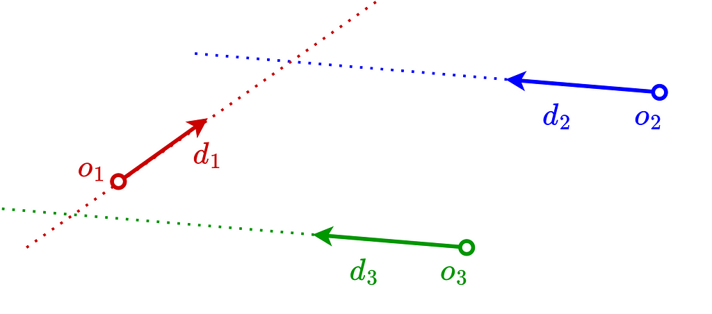
The 2D case is the easiest one. Typically, unless they’re exactly parallel, two 2D lines will always converge at a unique common point.
In the image below, r1 and r2 intersect. However, r3 doesn’t intersect any ray because it’s parallel to r2 and meets r1 behind its origin.
Solving the linear system
The linear system of equations Ax=b introduced above has n equations and 2 unknowns. Thus, in the 2D case we end up with a system of 2 equations and 2 unknowns, meaning we just have to invert the matrix A.

If the rays are parallel, the matrix A won’t be invertible because its two columns, d1 and -d2, will be collinear.
If you’re not interesting in t1 and t2 and just want to know if there’s an intersection, computing the determinant of A and comparing it against 0 is all you need.
If you’re not interesting in having both t1 and t2, e.g. if you’re looking for the actual 2D position of the intersection point, using Cramer’s rule is a smart trick. It expresses the solution using determinants of A and modified matrices, where one column of A is replaced by b.

3D Ray Intersection
Introduction
Unlike the 2D case, it’s highly unlikely for two 3D rays to intersect. For instance, trying to make two laser pointers held by two different people intersect is very challenging.
The linear system Ax=b ends up having 3 equations for 2 unknowns, making it unsolvable unless there’s redundancy within the equations.
Least-Squares
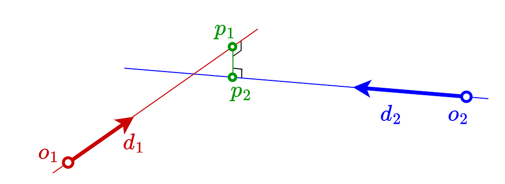
Given the absence of a solution in most cases, the shortest line segment between both rays can be viewed as their intersection. Let’s denote p1 and p2 as the endpoints of this optimal segment, located on r1 and r2 respectively.
Our task now transforms into a least-squares minimization problem. Its formulation is straightforward given that Ax-b already represents the vector between p2 and p1.
It’s a well-known problem. Zeroing the gradient at the optimum gives us the solution using the pseudo-inverse matrix, which is a convenient way to build a square and thus invertible matrix.
Orthogonality
While it appears on the diagram above that the shortest segment is perpendicular to both rays, we have yet to formally prove this, even-though it sounds intuitive.
The zero gradient also implies that the dot product between the segment defined by p1 and p2 and both ray directions d1 and d2 is zero, which proves the orthogonality.
Alternative Linear System
The Least-Squares approach works perfectly fine, but we can also introduce a third unknown variable to make our linear system solvable.
Given that the vectors d1, d2 and p2-p1 constitute an orthogonal basis, we can build an orthogonal frame with o1 as the origin. The points p1 and p2 can then be derived by expressing the local coordinates of o2 with respect to this frame.
We’ll denote the signed length of the segment p2-p1 as δ. Note that the direction of the segment is given by the cross product between both ray directions.
The determinant of a 3×3 matrix can be derived via the scalar triple product, which involves the dot product of one column with the cross product of the other two.

In our case, simplifying the determinant equation is straightforward as the second column is already a cross product. Note that inserting the cross product as the final column would have resulted in the negation of the norm instead.
Solving with Cramer’s rule gives us the optimal t1 and t2 , but also the signed length δ of the shortest segment.

If you love clean equations, you can re-order and swap columns to remove minus signs and make it look better!

Intersection Point
The intersection point can be defined as the middle of the shortest segment, i.e. 0.5(p1+p2).
Conclusion
I hope you enjoyed reading this article and that it gave you more insights on how to intersect 2D or 3D rays!
Intersect 3D Rays (Closest Point) was originally published in Towards Data Science on Medium, where people are continuing the conversation by highlighting and responding to this story.
Let’s unravel the math behind 3D rays and demonstrate that it’s not significantly more challenging than the conventional 2D case.

1. Introduction
Motivation
In fields like computer graphics, autonomous vehicle navigation or augmented reality, where immersive experiences are created through the manipulation of 3D environments, a deep understanding of ray intersection and triangulation algorithms empowers data scientists to craft lifelike simulations and interactive virtual worlds.
It also demonstrates that mathematical principles such as pseudo-inverse matrices, least squares optimization, Cramer’s rule or triple scalar products aren’t just theoretical; they’re practical tools for solving real-world problems!
Ray Definition
A Ray starts from a given position and extends infinitely in a given direction, just like a laser beam or a ray of light.
Think of a ray as a one-way street with a fixed starting point, while a line is like a two-way street that stretches endlessly in both directions.
Mathematically, a ray is defined by its origin o and direction d. Since it’s a 1D space, any point along the ray is parametrized by its positive distance (or time) t with respect to the origin.
Ray Intersection
Finding the intersection of two rays r1 and r2 means finding the two parameters t1 and t2, respectively on the first and second ray, that result in the exact same point in space.
An interesting point to note is that we haven’t specified the dimension of the space in which our ray lives. It could be 2D, like a line drawn on a piece of paper, 3D like a laser beam, or even exist in higher dimensions!
Since we’re looking for the values of t1 and t2, let’s concatenate them in a colum vector x. It allows us to vectorize this equation into the canonical linear system Ax=b. For better clarity, there’s an annotation below each term indicating the shape of the matrix or vector, with n being the dimension of the space in which the ray is defined.
N.B. The matrix A is built by concatenating side by side the two directions as column vectors, with the second one being flipped.
Solving Ax=b gives us t1 and t2. However, if either of these parameters is negative, it indicates that the intersection point lies behind one of the ray origins, meaning there’s no intersection between both rays.
2. 2D Ray Intersection
Introduction
The 2D case is the easiest one. Typically, unless they’re exactly parallel, two 2D lines will always converge at a unique common point.
In the image below, r1 and r2 intersect. However, r3 doesn’t intersect any ray because it’s parallel to r2 and meets r1 behind its origin.
Solving the linear system
The linear system of equations Ax=b introduced above has n equations and 2 unknowns. Thus, in the 2D case we end up with a system of 2 equations and 2 unknowns, meaning we just have to invert the matrix A.
If the rays are parallel, the matrix A won’t be invertible because its two columns, d1 and -d2, will be collinear.
If you’re not interesting in t1 and t2 and just want to know if there’s an intersection, computing the determinant of A and comparing it against 0 is all you need.
If you’re not interesting in having both t1 and t2, e.g. if you’re looking for the actual 2D position of the intersection point, using Cramer’s rule is a smart trick. It expresses the solution using determinants of A and modified matrices, where one column of A is replaced by b.
3D Ray Intersection
Introduction
Unlike the 2D case, it’s highly unlikely for two 3D rays to intersect. For instance, trying to make two laser pointers held by two different people intersect is very challenging.
The linear system Ax=b ends up having 3 equations for 2 unknowns, making it unsolvable unless there’s redundancy within the equations.
Least-Squares
Given the absence of a solution in most cases, the shortest line segment between both rays can be viewed as their intersection. Let’s denote p1 and p2 as the endpoints of this optimal segment, located on r1 and r2 respectively.
Our task now transforms into a least-squares minimization problem. Its formulation is straightforward given that Ax-b already represents the vector between p2 and p1.
It’s a well-known problem. Zeroing the gradient at the optimum gives us the solution using the pseudo-inverse matrix, which is a convenient way to build a square and thus invertible matrix.
Orthogonality
While it appears on the diagram above that the shortest segment is perpendicular to both rays, we have yet to formally prove this, even-though it sounds intuitive.
The zero gradient also implies that the dot product between the segment defined by p1 and p2 and both ray directions d1 and d2 is zero, which proves the orthogonality.
Alternative Linear System
The Least-Squares approach works perfectly fine, but we can also introduce a third unknown variable to make our linear system solvable.
Given that the vectors d1, d2 and p2-p1 constitute an orthogonal basis, we can build an orthogonal frame with o1 as the origin. The points p1 and p2 can then be derived by expressing the local coordinates of o2 with respect to this frame.
We’ll denote the signed length of the segment p2-p1 as δ. Note that the direction of the segment is given by the cross product between both ray directions.
The determinant of a 3×3 matrix can be derived via the scalar triple product, which involves the dot product of one column with the cross product of the other two.
In our case, simplifying the determinant equation is straightforward as the second column is already a cross product. Note that inserting the cross product as the final column would have resulted in the negation of the norm instead.
Solving with Cramer’s rule gives us the optimal t1 and t2 , but also the signed length δ of the shortest segment.
If you love clean equations, you can re-order and swap columns to remove minus signs and make it look better!
Intersection Point
The intersection point can be defined as the middle of the shortest segment, i.e. 0.5(p1+p2).
Conclusion
I hope you enjoyed reading this article and that it gave you more insights on how to intersect 2D or 3D rays!
Intersect 3D Rays (Closest Point) was originally published in Towards Data Science on Medium, where people are continuing the conversation by highlighting and responding to this story.
Denial of responsibility! Techno Blender is an automatic aggregator of the all world’s media. In each content, the hyperlink to the primary source is specified. All trademarks belong to their rightful owners, all materials to their authors. If you are the owner of the content and do not want us to publish your materials, please contact us by email – [email protected]. The content will be deleted within 24 hours.