
Introducing tidyverse — the Solution for Data Analysts Struggling with R | by Charlotte Patola | Jun, 2022
The tidyverse library provides an easy and “SQL-like way” of doing data wrangling in R
I had just started my university studies in Computer Science and was eager to learn the secrets of data analytics with R. After a few months of calculating answers to statistical questions, to my disappointment, I realized that I still was not able to write more than a few lines of code without consulting the course R Handbook. All the square brackets, commas, and dollar signs got mixed up in my head and even the simple task of filtering rows of a data frame felt far from straightforward.
I came to the point where I thought that R and I were just not compatible and decided to turn to python and pandas whenever I needed to analyze data.
Do you also have trouble getting your head around R? If this is the case, I have good news for you. There is an easier and more intuitive way to work with R: the tidyverse library! It’s not just another set of tools. It’s a completely different way of doing data analytics in R.
My first real encounter with tidyverse was when I started to work for my current employer. They did most of their advanced analytics in R. As I acknowledged my poor R skills, I was surprised to hear my colleague respond that it didn’t matter, as they use tidyverse anyway!
tidyverse is a collection of R packages that are developed especially for the needs of data analysts and scientists. The collection includes logic for many different types of scenarios, for example, time intelligence, data wrangling, and string manipulation.
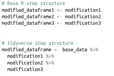
Functions included in the packages are designed to be as intuitive as possible to use and require a minimal amount of tuning. One example is the pipe, ie. the %>%-sign. The pipe’s function is to link together different data wrangling steps without having to save the results of each step into different variables. This makes the code both tidier and faster to write. Have a look at the difference in logic in the pseudocode below.
Another example is the SQL-like naming of common data frame modification functions. To filter rows in a data frame, you use the filter function, and to select specific columns, you use the select function.
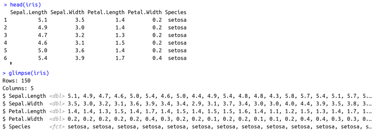
Yet another good example is the glimpse function. Glimpse’s main benefit is that it prints column names vertically. By contrast, head — the base R function for inspecting data — prints them horizontally. With glimpse, all column names will fit the print area, no matter how many there are.
One of the best ways to get to know tidyverse’s benefits is to try some basic data wrangling exercises; select some columns, filter some rows and manipulate some values. Let’s try these things with the built-in iris dataset.
Before getting started with the wrangling, download and load tidyverse. This might take a few minutes.
install.packages("tidyverse")
library(tidyverse)
Create New Data: tribble
The iris dataset is quite limited, with information merely on the species and dimensions of the flower. Let’s enrich the data with a link to each species’ Wikipedia page. We can do this by creating a new data frame with the tribble function.
Column names are marked with a ~before the column name and the content of each column is separated with a comma.
iris_wikipedia <- tribble(
~ Species,
~ Wikipedia,
'setosa',
'https://en.wikipedia.org/wiki/Iris_setosa',
'versicolor',
'https://en.wikipedia.org/wiki/Iris_versicolor',
'virginica',
'https://en.wikipedia.org/wiki/Iris_virginica'
)
Combine with Other Data: join
Now when we have our Wikipedia data, we can combine it with the iris dataset with a join. tidyverse provides several types of joins, but we go for a left join. The Species column will act as a key in the join and we have to make sure the data type is the same in both datasets. In the iris dataset, the data type is factor, while it is character in iris_wikipedia.
Let’s change the data type of the latter with the mutate function (a more detailed description of this function is found further below).
iris_wikipedia <- tribble(
~ Species,
~ Wikipedia,
'setosa',
'https://en.wikipedia.org/wiki/Iris_setosa',
'versicolor',
'https://en.wikipedia.org/wiki/Iris_versicolor',
'virginica',
'https://en.wikipedia.org/wiki/Iris_virginica'
) %>%
mutate(Species = as.factor(Species))
After defining the original iris dataset as our starting point, we take it and send it to the left_join function with the help of tidyverse’s pipe function. If the datasets contain columns with the same name and data type, only the name of the new dataset needs to be supplied to left_join. If the column names differ, the keys are provided as a vector assigned to the by parameter:by = c("column_name_in_base_dataset" = "column_name_in_new_dataset")
our_wrangled_data <- iris %>%
left_join(iris_wikipedia)
Filter Rows: filter
Let’s say that we only want to include the species “sentosa” in our analysis. We do it by piping the output of the previous step to the filter function. Note that double equal signs are used. Not equal to is defined as !=.
our_wrangled_data <- iris %>%
left_join(iris_wikipedia) %>%
filter(Species == "setosa")
Select Columns: select
We are only interested in sepal and Wikipedia-related data and therefore select only those columns. The select function can be used both to select columns we want or don’t want. In the latter case, we just add a minus sign before the column names: select(-unwanted_column_name).
our_wrangled_data <- iris %>%
left_join(iris_wikipedia) %>%
filter(Species == "setosa") %>%
select(Sepal.Length, Sepal.Width, Wikipedia)
Create a New Column or Modify an Existing: mutate
The function mutate can be used both to change the content of an existing column and to create a new column with a specified logic.
In this example, we create the new column Long.Sepal that gets the boolean value true if the row’s Sepal.Length is longer than the average of all setosa sepal lengths. If we would have named the new column Sepal.Length, it would have overwritten the existing Sepal.Length column. This is what we did with the Species column of iris_wikipedia before the join.
our_wrangled_data <- iris %>%
left_join(iris_wikipedia) %>%
filter(Species == "setosa") %>%
select(Sepal.Length, Sepal.Width, Wikipedia) %>%
mutate(Long.Sepal = if_else(Sepal.Length > mean(Sepal.Length),
TRUE,
FALSE))
In tidyverse, group_by can be used both to create a summarised data frame (group by in SQL) and to create a summarised column, while preserving the original data frame (window functions in SQL). In the former case, group_by is used together with summarise. In the latter it is — usually — used together with mutate and then ungroup, which removes the group_by environment, so that possible subsequent functions are applied all over the data frame and not only on the grouped data.
Let’s try both versions. We start with the basic group_by in order to summarise information on average Sepal.Length for observations based on their Long.Sepal status.
our_wrangled_data <- iris %>%
left_join(iris_wikipedia) %>%
filter(Species == "setosa") %>%
select(Sepal.Length, Sepal.Width, Wikipedia) %>%
mutate(Long.Sepal = if_else(Sepal.Length > mean(Sepal.Length),
TRUE,
FALSE)) %>%
group_by(Long.Sepal) %>%
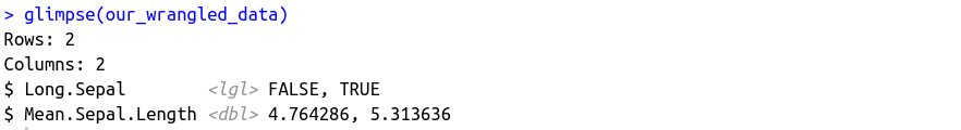
summarise(Mean.Sepal.Length = mean(Sepal.Length))
We get the following output:
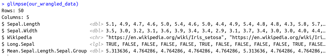
To get the same aggregated mean information, but preserve the data frame structure, we create a new column with mutate, after having used the group_by function. This creates the same means as with the summarise function, but the amount of rows remains the same.
As this is the last wrangling step, ungroup is not required. However, in case we would later add more transformation steps, it is a good idea to include it already now, so it won’t get forgotten later on.
our_wrangled_data <- iris %>%
left_join(iris_wikipedia) %>%
filter(Species == "setosa") %>%
select(Sepal.Length, Sepal.Width, Wikipedia) %>%
mutate(Long.Sepal = if_else(Sepal.Length > mean(Sepal.Length),
TRUE,
FALSE)) %>%
group_by(Long.Sepal) %>%
mutate(Mean.Sepal.Length.Sepal.Group = mean(Sepal.Length)) %>%
ungroup()
The output looks like this:
With the help of these and related functions, I estimate that I get 70 % of my data wrangling done. One main thing that is missing is data imports. I mainly use Snowflake and Azure Storage connectors, but R connectors exist for most of the widely used data storage solutions.
The tidyverse library provides an easy and “SQL-like way” of doing data wrangling in R

I had just started my university studies in Computer Science and was eager to learn the secrets of data analytics with R. After a few months of calculating answers to statistical questions, to my disappointment, I realized that I still was not able to write more than a few lines of code without consulting the course R Handbook. All the square brackets, commas, and dollar signs got mixed up in my head and even the simple task of filtering rows of a data frame felt far from straightforward.
I came to the point where I thought that R and I were just not compatible and decided to turn to python and pandas whenever I needed to analyze data.
Do you also have trouble getting your head around R? If this is the case, I have good news for you. There is an easier and more intuitive way to work with R: the tidyverse library! It’s not just another set of tools. It’s a completely different way of doing data analytics in R.
My first real encounter with tidyverse was when I started to work for my current employer. They did most of their advanced analytics in R. As I acknowledged my poor R skills, I was surprised to hear my colleague respond that it didn’t matter, as they use tidyverse anyway!
tidyverse is a collection of R packages that are developed especially for the needs of data analysts and scientists. The collection includes logic for many different types of scenarios, for example, time intelligence, data wrangling, and string manipulation.
Functions included in the packages are designed to be as intuitive as possible to use and require a minimal amount of tuning. One example is the pipe, ie. the %>%-sign. The pipe’s function is to link together different data wrangling steps without having to save the results of each step into different variables. This makes the code both tidier and faster to write. Have a look at the difference in logic in the pseudocode below.
Another example is the SQL-like naming of common data frame modification functions. To filter rows in a data frame, you use the filter function, and to select specific columns, you use the select function.
Yet another good example is the glimpse function. Glimpse’s main benefit is that it prints column names vertically. By contrast, head — the base R function for inspecting data — prints them horizontally. With glimpse, all column names will fit the print area, no matter how many there are.
One of the best ways to get to know tidyverse’s benefits is to try some basic data wrangling exercises; select some columns, filter some rows and manipulate some values. Let’s try these things with the built-in iris dataset.
Before getting started with the wrangling, download and load tidyverse. This might take a few minutes.
install.packages("tidyverse")
library(tidyverse)
Create New Data: tribble
The iris dataset is quite limited, with information merely on the species and dimensions of the flower. Let’s enrich the data with a link to each species’ Wikipedia page. We can do this by creating a new data frame with the tribble function.
Column names are marked with a ~before the column name and the content of each column is separated with a comma.
iris_wikipedia <- tribble(
~ Species,
~ Wikipedia,
'setosa',
'https://en.wikipedia.org/wiki/Iris_setosa',
'versicolor',
'https://en.wikipedia.org/wiki/Iris_versicolor',
'virginica',
'https://en.wikipedia.org/wiki/Iris_virginica'
)
Combine with Other Data: join
Now when we have our Wikipedia data, we can combine it with the iris dataset with a join. tidyverse provides several types of joins, but we go for a left join. The Species column will act as a key in the join and we have to make sure the data type is the same in both datasets. In the iris dataset, the data type is factor, while it is character in iris_wikipedia.
Let’s change the data type of the latter with the mutate function (a more detailed description of this function is found further below).
iris_wikipedia <- tribble(
~ Species,
~ Wikipedia,
'setosa',
'https://en.wikipedia.org/wiki/Iris_setosa',
'versicolor',
'https://en.wikipedia.org/wiki/Iris_versicolor',
'virginica',
'https://en.wikipedia.org/wiki/Iris_virginica'
) %>%
mutate(Species = as.factor(Species))
After defining the original iris dataset as our starting point, we take it and send it to the left_join function with the help of tidyverse’s pipe function. If the datasets contain columns with the same name and data type, only the name of the new dataset needs to be supplied to left_join. If the column names differ, the keys are provided as a vector assigned to the by parameter:by = c("column_name_in_base_dataset" = "column_name_in_new_dataset")
our_wrangled_data <- iris %>%
left_join(iris_wikipedia)
Filter Rows: filter
Let’s say that we only want to include the species “sentosa” in our analysis. We do it by piping the output of the previous step to the filter function. Note that double equal signs are used. Not equal to is defined as !=.
our_wrangled_data <- iris %>%
left_join(iris_wikipedia) %>%
filter(Species == "setosa")
Select Columns: select
We are only interested in sepal and Wikipedia-related data and therefore select only those columns. The select function can be used both to select columns we want or don’t want. In the latter case, we just add a minus sign before the column names: select(-unwanted_column_name).
our_wrangled_data <- iris %>%
left_join(iris_wikipedia) %>%
filter(Species == "setosa") %>%
select(Sepal.Length, Sepal.Width, Wikipedia)
Create a New Column or Modify an Existing: mutate
The function mutate can be used both to change the content of an existing column and to create a new column with a specified logic.
In this example, we create the new column Long.Sepal that gets the boolean value true if the row’s Sepal.Length is longer than the average of all setosa sepal lengths. If we would have named the new column Sepal.Length, it would have overwritten the existing Sepal.Length column. This is what we did with the Species column of iris_wikipedia before the join.
our_wrangled_data <- iris %>%
left_join(iris_wikipedia) %>%
filter(Species == "setosa") %>%
select(Sepal.Length, Sepal.Width, Wikipedia) %>%
mutate(Long.Sepal = if_else(Sepal.Length > mean(Sepal.Length),
TRUE,
FALSE))
In tidyverse, group_by can be used both to create a summarised data frame (group by in SQL) and to create a summarised column, while preserving the original data frame (window functions in SQL). In the former case, group_by is used together with summarise. In the latter it is — usually — used together with mutate and then ungroup, which removes the group_by environment, so that possible subsequent functions are applied all over the data frame and not only on the grouped data.
Let’s try both versions. We start with the basic group_by in order to summarise information on average Sepal.Length for observations based on their Long.Sepal status.
our_wrangled_data <- iris %>%
left_join(iris_wikipedia) %>%
filter(Species == "setosa") %>%
select(Sepal.Length, Sepal.Width, Wikipedia) %>%
mutate(Long.Sepal = if_else(Sepal.Length > mean(Sepal.Length),
TRUE,
FALSE)) %>%
group_by(Long.Sepal) %>%
summarise(Mean.Sepal.Length = mean(Sepal.Length))
We get the following output:
To get the same aggregated mean information, but preserve the data frame structure, we create a new column with mutate, after having used the group_by function. This creates the same means as with the summarise function, but the amount of rows remains the same.
As this is the last wrangling step, ungroup is not required. However, in case we would later add more transformation steps, it is a good idea to include it already now, so it won’t get forgotten later on.
our_wrangled_data <- iris %>%
left_join(iris_wikipedia) %>%
filter(Species == "setosa") %>%
select(Sepal.Length, Sepal.Width, Wikipedia) %>%
mutate(Long.Sepal = if_else(Sepal.Length > mean(Sepal.Length),
TRUE,
FALSE)) %>%
group_by(Long.Sepal) %>%
mutate(Mean.Sepal.Length.Sepal.Group = mean(Sepal.Length)) %>%
ungroup()
The output looks like this:
With the help of these and related functions, I estimate that I get 70 % of my data wrangling done. One main thing that is missing is data imports. I mainly use Snowflake and Azure Storage connectors, but R connectors exist for most of the widely used data storage solutions.
Denial of responsibility! Techno Blender is an automatic aggregator of the all world’s media. In each content, the hyperlink to the primary source is specified. All trademarks belong to their rightful owners, all materials to their authors. If you are the owner of the content and do not want us to publish your materials, please contact us by email – [email protected]. The content will be deleted within 24 hours.