Introduction to Instrumental Variables Estimation | by Sachin Date | Aug, 2022

We’ll learn about Instrumental Variables, and how to use them for estimating a linear regression model

In this article, we’ll learn about an ingenious technique for estimating linear regression models using an artifact called the Instrumental Variable.

Instrumental Variables (IV) based estimation allows the regression modeler to deal with a serious situation that bedevils a large fraction of regression models, one where one or more regression variables turn out to be correlated with the error term of the model. In other words, the regression variables are endogenous.

Ordinary Least-Squares based estimation of a model containing endogenous variables yields biased estimates of the regression coefficients due to a phenomena known as Omitted Variable Bias. Functionally, this bias in coefficients leads to a whole host of practical problems for the experimenter and may bring into question the usefulness of the entire experiment.

In IV estimation, we use one or more Instrumental Variables (Instruments) in place of the suspected endogenous variables, and we estimate the resulting model using a modified form of least-squares known as 2-stage least-squares (2SLS in short).

In the rest of the article, we’ll show how instrumental variables can be used to mitigate the effects of endogeneity, and we’ll illustrate the use of IVs using an example.

In the previous article, we learnt about exogenous and endogenous variables. Let’s quickly recap the concepts.

Consider the following linear model:

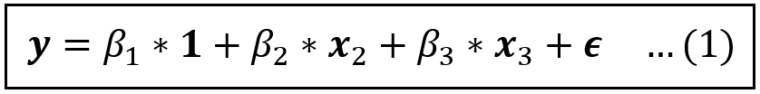
In the above equation, y is the dependent variable, x_2 and x_3 are explanatory variables and ϵ is the error term which captures the variance in y that x_2 and x_3 have not been able to “explain”. For a data set containing n rows, 1, y, x_2, x_3, ϵ are all column vectors of size [n x 1] — hence the bold notation. We’ll drop the 1 (which is a vector of 1s) from subsequent equations for brevity.

If one or more regression variables, say x_3, is endogenous, i.e., it is correlated with the error term, the the OLS estimator is not consistent. The coefficient estimates of all variables, not just of x_3, are biased away from the true values due to a phenomenon known as the Omitted Variable Bias.

In the face of endogeneity, this estimation bias never goes away no matter how big or how well-balanced is your data set.

When faced with endogeneity in your model, you have the following options:

1. If the endogeneity is suspected to be small, you may simply accept it and the consequent bias in coefficient estimates.
2. You may choose suitable proxy variables for the unobservable factors hiding within the error term that you are suspecting the endogenous variables to be correlated with.
3. If the suspected endogenous variables are time invariant, i.e., their values do not change with time, then time-differencing the model once, will subtract them out. It’s a strategy that works primarily in panel data models.
4. You may use Instrumental Variables (IVs) in place of the suspected endogenous variables and estimate the “instrumented” model using an IV estimation technique such as 2-stage Least Squares.

Let’s learn more about how to use IVs.

Consider once again the model in Eq (1):

Before we begin, let’s note the following:

If x_2 and x_3 are both exogenous, the OLS estimator is consistent and all coefficient estimates it produces are unbiased. There is no need for IV based estimation.

But now suppose x_3 is endogenous. We’ll conceptually look at the variance of x_3 as being made of two parts:

1. A chunk that is uncorrelated with ϵ. This is the part of x_3 that is, in fact, exogenous.
2. A second chunk that is correlated with ϵ. This is the part of x_3 that is endogenous.

The key intuition behind Instrumental Variables

If we are able to somehow separate out the exogenous portion of x_3 and replace x_3 with this exogenous chunk while at the same time leaving out from the model the endogenous portion of x_3, the resulting model would contain only exogenous explanatory variables and it can be consistently estimated using OLS. This is the key intuition behind using Instrumental Variables in linear models.

To that effect, suppose we are able to identify a regression variable z_3 such that z_3 has the following two properties:

1. z_3 is correlated with x_3. Notation-wise: Cov(z_3, x_3) != 0. This is known as the relevance condition for including z_3. Simply put, z_3 should be relevant to x_3.
2. z_3 is uncorrelated with the error term, i.e. E(ϵ|x_3)= 0 or constant, and E(ϵ*x_3)=0. This is known as the exogeneity condition for using z_3.

If z_3 satisfies the relevance condition and the exogeneity condition, z_3 is known as the Instrumental Variable or the Instrument for x_2.

But first, let’s examine a subtle point about z_3.

Since z_3 is correlated with x_3, we can express x_3 as a linear combination of z_3 and an error term as follows:

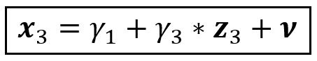
However, z_3 could also be correlated with x_2. Such kind of collinearity amongst regression variables is very common in real settings. Due to this collinearity, x_2 may be influencing x_3 via z_3 and in the above equation, γ_3 captures not just the effect of z_3 on x_3, but also x_2 on x_3.

We may want to isolate out the effect of x_2 on x_3 so that the main effect of z_3 on x_3 shows through. For that, we must regress x_3 not just on z_3, but also on both x_2:

As before, x_3, x_2, z_3, and the error term ν are column vectors of size [n x 1]. Also, in Eq (1a), x_2 and z_3 are exogenous i.e. they are uncorrelated with ν.

Substituting Eq (1a) into Eq (1):

The green bit can be absorbed into a new intercept β*_1. Similarly, we’ll substitute (β_2+β_3* γ_2) with a new coefficient β*_2, and (β_3* γ_3) with β*_3, and the composite error term (β_3*ν)+ϵ can be substituted by ϵ*.

With these substitutions, the regression model in Eq (1) is transformed into the following model:

Recollect that x_2 and z_3 are each assumed to be uncorrelated ν and ϵ. Hence they are also uncorrelated with the composite error ϵ*. Thus, in Eq (1b), all variables on the R.H.S. are exogenous and Eq (1b) can be estimated consistently using OLS.

Consider the following treatment-effect model of lifetime earnings regressed on whether the person attended an Ivy League school:

The boolean variable Attended_Ivy_League is obviously endogenous. Whether the person attended an Ivy League school depends on socioeconomic factors and person-specific factors such as ability and a drive to succeed in life which cannot be measured but which also directly influence lifetime earnings. Hence these unobservable variables are hidden within the error term and they are also correlated with Attended_Ivy_League, making Attended_Ivy_League endogenous. Estimation using OLS will lead to biased estimates of β_1 and β_2.

It’s hard to imagine how a greater drive to succeed will result in a systematically lesser chance of Ivy League attendance. Ditto for other factors such as ability. Hence, we assume a positive correlation between the hidden factors in ϵ and Attended_Ivy_League leading to a positive bias on β_1 and β_2, in turn leading to the experimenter’s overestimating the effect of Ivy League attendance on lifetime earnings.

Clearly, a solution a needed for this problem. Let’s try to identify a variable that is correlated with Attended_Ivy_League but uncorrelated with the error term. One such variable is Legacy, i.e. whether the person’s parents or grandparents attended an Ivy League school. Data shows that there is a correlation between a person’s Legacy status and whether the person enrolled in the same Ivy League school. This satisfies the relevance condition. Moreover, whether the person’s parents or grandparents attended an Ivy League school does not seem to be directly correlated with factors such as the person’s ability and motivation, thereby satisfying the exogeneity condition. Thus we have:

Cov(Legacy, Attended_Ivy_League) != 0

Cov(Legacy, ϵ) = 0

Thus, we appoint Legacy as the instrument for Attended_Ivy_League. We’ll estimate the following instrumented model instead of the original model:

This instrumented model can be consistently estimated using OLS and one would get unbiased estimates of β*_1 and β*_2. Note that β*_2 is the effect of Legacy, and not Attended_Ivy_League on Lifetime_Earnings. But we have seen that β_2 cannot be estimated reliably anyway. So we must accept β*_2 as the representative of β_2. Incidentally, estimation software will report β*_2 as the coefficient of the original endogenous variable Attended_Ivy_League, and not of Legacy which is a good thing.

We’ll learn about Instrumental Variables, and how to use them for estimating a linear regression model

In this article, we’ll learn about an ingenious technique for estimating linear regression models using an artifact called the Instrumental Variable.

Instrumental Variables (IV) based estimation allows the regression modeler to deal with a serious situation that bedevils a large fraction of regression models, one where one or more regression variables turn out to be correlated with the error term of the model. In other words, the regression variables are endogenous.

Ordinary Least-Squares based estimation of a model containing endogenous variables yields biased estimates of the regression coefficients due to a phenomena known as Omitted Variable Bias. Functionally, this bias in coefficients leads to a whole host of practical problems for the experimenter and may bring into question the usefulness of the entire experiment.

In IV estimation, we use one or more Instrumental Variables (Instruments) in place of the suspected endogenous variables, and we estimate the resulting model using a modified form of least-squares known as 2-stage least-squares (2SLS in short).

In the rest of the article, we’ll show how instrumental variables can be used to mitigate the effects of endogeneity, and we’ll illustrate the use of IVs using an example.

In the previous article, we learnt about exogenous and endogenous variables. Let’s quickly recap the concepts.

Consider the following linear model:

In the above equation, y is the dependent variable, x_2 and x_3 are explanatory variables and ϵ is the error term which captures the variance in y that x_2 and x_3 have not been able to “explain”. For a data set containing n rows, 1, y, x_2, x_3, ϵ are all column vectors of size [n x 1] — hence the bold notation. We’ll drop the 1 (which is a vector of 1s) from subsequent equations for brevity.

If one or more regression variables, say x_3, is endogenous, i.e., it is correlated with the error term, the the OLS estimator is not consistent. The coefficient estimates of all variables, not just of x_3, are biased away from the true values due to a phenomenon known as the Omitted Variable Bias.

In the face of endogeneity, this estimation bias never goes away no matter how big or how well-balanced is your data set.

When faced with endogeneity in your model, you have the following options:

1. If the endogeneity is suspected to be small, you may simply accept it and the consequent bias in coefficient estimates.
2. You may choose suitable proxy variables for the unobservable factors hiding within the error term that you are suspecting the endogenous variables to be correlated with.
3. If the suspected endogenous variables are time invariant, i.e., their values do not change with time, then time-differencing the model once, will subtract them out. It’s a strategy that works primarily in panel data models.
4. You may use Instrumental Variables (IVs) in place of the suspected endogenous variables and estimate the “instrumented” model using an IV estimation technique such as 2-stage Least Squares.

Let’s learn more about how to use IVs.

Consider once again the model in Eq (1):

Before we begin, let’s note the following:

If x_2 and x_3 are both exogenous, the OLS estimator is consistent and all coefficient estimates it produces are unbiased. There is no need for IV based estimation.

But now suppose x_3 is endogenous. We’ll conceptually look at the variance of x_3 as being made of two parts:

1. A chunk that is uncorrelated with ϵ. This is the part of x_3 that is, in fact, exogenous.
2. A second chunk that is correlated with ϵ. This is the part of x_3 that is endogenous.

The key intuition behind Instrumental Variables

If we are able to somehow separate out the exogenous portion of x_3 and replace x_3 with this exogenous chunk while at the same time leaving out from the model the endogenous portion of x_3, the resulting model would contain only exogenous explanatory variables and it can be consistently estimated using OLS. This is the key intuition behind using Instrumental Variables in linear models.

To that effect, suppose we are able to identify a regression variable z_3 such that z_3 has the following two properties:

1. z_3 is correlated with x_3. Notation-wise: Cov(z_3, x_3) != 0. This is known as the relevance condition for including z_3. Simply put, z_3 should be relevant to x_3.
2. z_3 is uncorrelated with the error term, i.e. E(ϵ|x_3)= 0 or constant, and E(ϵ*x_3)=0. This is known as the exogeneity condition for using z_3.

If z_3 satisfies the relevance condition and the exogeneity condition, z_3 is known as the Instrumental Variable or the Instrument for x_2.

But first, let’s examine a subtle point about z_3.

Since z_3 is correlated with x_3, we can express x_3 as a linear combination of z_3 and an error term as follows:

However, z_3 could also be correlated with x_2. Such kind of collinearity amongst regression variables is very common in real settings. Due to this collinearity, x_2 may be influencing x_3 via z_3 and in the above equation, γ_3 captures not just the effect of z_3 on x_3, but also x_2 on x_3.

We may want to isolate out the effect of x_2 on x_3 so that the main effect of z_3 on x_3 shows through. For that, we must regress x_3 not just on z_3, but also on both x_2:

As before, x_3, x_2, z_3, and the error term ν are column vectors of size [n x 1]. Also, in Eq (1a), x_2 and z_3 are exogenous i.e. they are uncorrelated with ν.

Substituting Eq (1a) into Eq (1):

The green bit can be absorbed into a new intercept β*_1. Similarly, we’ll substitute (β_2+β_3* γ_2) with a new coefficient β*_2, and (β_3* γ_3) with β*_3, and the composite error term (β_3*ν)+ϵ can be substituted by ϵ*.

With these substitutions, the regression model in Eq (1) is transformed into the following model:

Recollect that x_2 and z_3 are each assumed to be uncorrelated ν and ϵ. Hence they are also uncorrelated with the composite error ϵ*. Thus, in Eq (1b), all variables on the R.H.S. are exogenous and Eq (1b) can be estimated consistently using OLS.

Consider the following treatment-effect model of lifetime earnings regressed on whether the person attended an Ivy League school:

The boolean variable Attended_Ivy_League is obviously endogenous. Whether the person attended an Ivy League school depends on socioeconomic factors and person-specific factors such as ability and a drive to succeed in life which cannot be measured but which also directly influence lifetime earnings. Hence these unobservable variables are hidden within the error term and they are also correlated with Attended_Ivy_League, making Attended_Ivy_League endogenous. Estimation using OLS will lead to biased estimates of β_1 and β_2.

It’s hard to imagine how a greater drive to succeed will result in a systematically lesser chance of Ivy League attendance. Ditto for other factors such as ability. Hence, we assume a positive correlation between the hidden factors in ϵ and Attended_Ivy_League leading to a positive bias on β_1 and β_2, in turn leading to the experimenter’s overestimating the effect of Ivy League attendance on lifetime earnings.

Clearly, a solution a needed for this problem. Let’s try to identify a variable that is correlated with Attended_Ivy_League but uncorrelated with the error term. One such variable is Legacy, i.e. whether the person’s parents or grandparents attended an Ivy League school. Data shows that there is a correlation between a person’s Legacy status and whether the person enrolled in the same Ivy League school. This satisfies the relevance condition. Moreover, whether the person’s parents or grandparents attended an Ivy League school does not seem to be directly correlated with factors such as the person’s ability and motivation, thereby satisfying the exogeneity condition. Thus we have:

Cov(Legacy, Attended_Ivy_League) != 0

Cov(Legacy, ϵ) = 0

Thus, we appoint Legacy as the instrument for Attended_Ivy_League. We’ll estimate the following instrumented model instead of the original model:

This instrumented model can be consistently estimated using OLS and one would get unbiased estimates of β*_1 and β*_2. Note that β*_2 is the effect of Legacy, and not Attended_Ivy_League on Lifetime_Earnings. But we have seen that β_2 cannot be estimated reliably anyway. So we must accept β*_2 as the representative of β_2. Incidentally, estimation software will report β*_2 as the coefficient of the original endogenous variable Attended_Ivy_League, and not of Legacy which is a good thing.