Large Scale K-Means Clustering with Gradient Descent | by Sriram Kumar | Jun, 2022

Learning with sequential, mini-batch, and batch data

Clustering is an unsupervised form of a machine learning algorithm. It discovers sub-groups or patterns in the data. The K-Means algorithm is a simple and intuitive way to cluster data. When we apply the K-Means algorithm, we have to be mindful of dataset size and dimensionality. Either one of these can cause slow algorithmic convergence¹. In this article, we will explore gradient descent optimization and dimensionality reduction techniques to scale the K-Means algorithm for large datasets. I will also share some of my experimental results on popular image datasets.

In gradient descent optimization, we compute a derivative of the cost function and iteratively move in the opposite direction of the gradient until we reach an optimal value. This kind of optimization can be used to scale ML algorithms to train on large datasets by performing optimization on small batches of the dataset.

We may additionally apply dimensionality reduction techniques to the dataset to find better data representation and speed up clustering time. In the next section, we will see how K-Means can be performed with gradient descent learning.

The K-Means algorithm divides the dataset into groups of K distinct clusters. It uses a cost function that minimizes the sum of the squared distance between cluster centers and their assigned samples. The number of clusters is set based on domain knowledge or by some other strategy. The K-Means cost function² can be written as,

where sample x has a dimensionality d and N is the total number of samples in the dataset. The cluster centers are denoted by w. The standard K-Means algorithm alternates between cluster center estimation and distance computation between the cluster center and samples for a fixed number of iterations.

Next, we will see how to perform K-Means clustering with gradient descent optimization.

Standard K-Means algorithm can have slow convergence and memory-intensive computation on large datasets. We can address this problem with gradient descent optimization. For K-Means, the cluster center update² equation is written as,

where s(w) is the prototype closest to x in Euclidean space. The learning rate is set to the sample cluster count, i.e., the number of samples assigned to a particular cluster center². We stop this gradient optimization after a fixed number of iterations or when the change in K-Means cost is below some tolerance value. In batch gradient descent, we compute the gradient with the entire dataset. For large datasets, computing the gradient might be slow and inefficient.

Next, we will look at two variations of gradient descent to scale K-Means clustering.

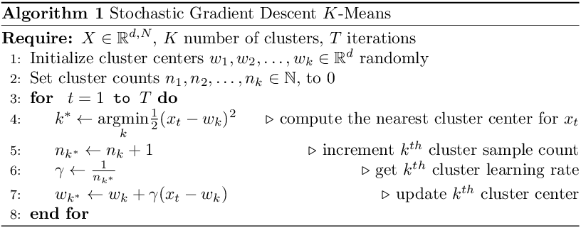
A variant of gradient descent that uses one sample to compute the gradient is called Stochastic Gradient Descent (SGD). As it performs the cluster update with only a single sample, it can be applied to online learning. In practice, we randomize our dataset and process one sample at a time. The learning rate is updated during each iteration, and for each cluster center³. This approach works well in practice. The pseudocode for SGD is shown below.

To visualize the K-Means SGD learning process, I created a toy dataset with two circular blobs that are linearly separable.

From the illustration, we see that the cluster center updates can be slow as only one sample is processed at a time. This may get worse when there are many distinct cluster centers to learn.

SGD may not find good cluster centers as only a single sample is used to compute the gradient. We can modify the gradient update step to use a batch size of M samples to compute the gradient. This variant is called mini-batch SGD. This has faster and smoother cost convergence than SGD. The reasoning behind mini-batch is that a subset of the data contains more information than a single sample while also being less likely to contain redundant examples found in the entire dataset¹. In practice, the mini-batch is sampled at random. The pseudocode for mini-batch SGD is shown below.

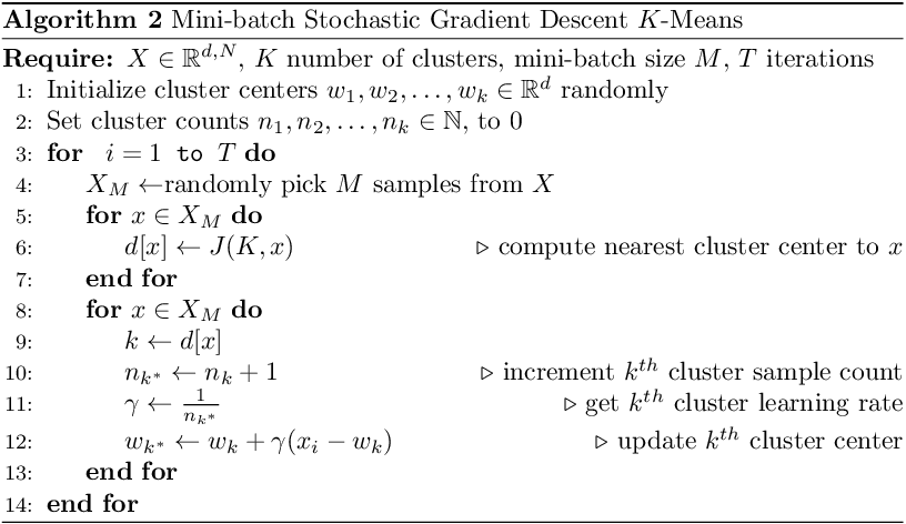
The algorithm is similar to SGD, except that we use M samples to compute the gradient at each iteration. The mini-batch size is a hyper-parameter to be tuned and its value can affect the performance of the algorithm.

Below is an illustration of the mini-batch SGD K-Means algorithm on the same toy dataset with a mini-batch of size 4. Compared to SGD, the cost convergence is faster. Both SGD and mini-batch SGD find good cluster centers and group the toy dataset well.

Next, we will go over two popular dimensionality reduction techniques and how they can improve and speed up the clustering workflow.

Dimensionality reduction can be seen as a feature selection and feature extraction step. The original data is mapped to a lower-dimensional space, which can help with the faster learning of clusters⁴. I experimented with the Principal Component Analysis (PCA) and Sparse Random Projection (SRP) methods.

Principal Component Analysis

PCA learns an embedding matrix that maximizes data variance. It is a data-dependent projection as the embedding matrix contains eigenvectors of the sample covariance matrix. A good overview of PCA with SVD is written by Jonathan Hui⁵.

Sparse Random Projection

SRP constructs a data-independent embedding matrix. Pairwise distances are preserved up to a factor in the lower dimension. Compared to the Gaussian random projection matrix, SRP enables faster data projection and is memory efficient. A detailed explanation and application of SRP are explained in this article by CJ Sullivan⁶.

To compare the different versions of K-Means, I ran clustering on the iris, USPS, and Fashion-MNIST datasets. These datasets contain small, medium, and large sample sizes with varying dimensionality. The sample distribution is uniform across classes for all three datasets. Below is a summary of the different datasets.

Randomly chosen samples are initialized as the cluster centers for all three K-Means algorithms. For batch gradient descent, I set the learning rate as 0.03/t for the iris dataset, and 0.1/t for the USPS and Fashion-MNIST datasets. For mini-batch SGD, I used 32 as the batch size. For both SGD and mini-batch SGD, I used the cluster assignment count as the learning rate. All datasets are scaled with a min-max scaler which scales each sample within the range [0,1]. Below is the formula used to scale the data.

I tried the standard scaler as well, which transforms data to have zero mean and unit standard deviation. For the above three datasets, I did not see a big difference in convergence speed or lower final cost.

Cost convergence of different gradient descent algorithms

When we compare the cost convergence on all three datasets, mini-batch SGD has a smoother and faster convergence. For the smaller iris dataset, SGD finds a lower cost than mini-batch SGD. This could be because the batch size of 32 might be too big. To see how mini-batch size affects convergence, I ran an experiment with 16, 32, 64, and 128 mini-batch sizes.

We see a big gap in the final cost between small and large mini-batch sizes. A mini-batch size of 16 produces the lowest final cost for all three datasets.

Relative clustering time reduction with dimensionality

The time reduction is a measure between standard K-Means with full dimensionality and mini-batch SGD K-Means with reduced dimensionality. I ran the mini-batch K-Means algorithm on the USPS and Fashion-MNIST datasets mapped with PCA and SRP with different dimensionalities. The dimensionality reduction computation step is not accounted for in the time calculation but only the data clustering time.

As expected, with more components, K-Means takes more time to converge to a lower cost. The time reduction trend decreases linearly with dimensionality.

Relative error of K-Means cost with dimensionality

The relative error is the difference in final cost between standard and mini-batch SGD K-Means. The standard K-Means was trained on the original dataset, and mini-batch K-Means was trained with varying dimensionalities. Below is the relative error visualized after PCA and SRP.

Random projections benefit when the original dimensionality is quite high. Compared to SRP, the relative cost difference with PCA reduces with more components (up to a point).

Code Snippet

We can use the scikit-learn API to create a simple pipeline for the clustering workflow. Below is a sample pipeline with PCA and mini-batch K-Means.

from sklearn.pipeline import Pipeline
from sklearn.preprocessing import MinMaxScaler
from sklearn.decomposition import PCA
from sklearn.cluster import MiniBatchKMeans
from sklearn.datasets import fetch_openml
# load dataset
X, y = fetch_openml('USPS', return_X_y=True, as_frame=False)# add methods to pipeline
steps = [
("scale_step", MinMaxScaler()),
("dimred_step", PCA(n_components=50)), 
("cluster_step", MiniBatchKMeans(n_clusters=10, batch_size=16))
]# create pipeline
clusterpipe = Pipeline(steps)# fit pipeline on data
clusterpipe.fit(X)

Both SGD versions work well with large-scale K-Means clustering. The mini-batch SGD converges faster and discovers better cluster centers than SGD on medium and large datasets. The mini-batch size is a hyper-parameter to be tuned and set based on the size of the dataset. Clustering benefits from dimensionality reduction approaches being memory efficient and having faster convergence. The speed and lower-cost trade-off curve visualizations are helpful when we are designing our machine learning pipeline.

[1] Sculley, D. (2010, April). Web-scale k-means clustering. In Proceedings of the 19th international conference on World wide web (pp. 1177–1178).

[2] Bottou, L., & Bengio, Y. (1994). Convergence properties of the k-means algorithms. Advances in neural information processing systems, 7.

[3] Bottou, L. (2012). Stochastic gradient descent tricks. In Neural networks: Tricks of the trade (pp. 421–436). Springer, Berlin, Heidelberg.

[4] Boutsidis, C., Zouzias, A., & Drineas, P. (2010). Random projections for k-means clustering. Advances in neural information processing systems, 23.

[5] Jonathan Hui. (2019). Machine Learning — Singular Value Decomposition (SVD) & Principal Component Analysis (PCA). Towards Data Science

[6] CJ Sullivan. (2021). Behind the scenes on the Fast Random Projection algorithm for generating graph embeddings. Towards Data Science

All images, unless otherwise noted, are by the author.

Learning with sequential, mini-batch, and batch data

Clustering is an unsupervised form of a machine learning algorithm. It discovers sub-groups or patterns in the data. The K-Means algorithm is a simple and intuitive way to cluster data. When we apply the K-Means algorithm, we have to be mindful of dataset size and dimensionality. Either one of these can cause slow algorithmic convergence¹. In this article, we will explore gradient descent optimization and dimensionality reduction techniques to scale the K-Means algorithm for large datasets. I will also share some of my experimental results on popular image datasets.

In gradient descent optimization, we compute a derivative of the cost function and iteratively move in the opposite direction of the gradient until we reach an optimal value. This kind of optimization can be used to scale ML algorithms to train on large datasets by performing optimization on small batches of the dataset.

We may additionally apply dimensionality reduction techniques to the dataset to find better data representation and speed up clustering time. In the next section, we will see how K-Means can be performed with gradient descent learning.

The K-Means algorithm divides the dataset into groups of K distinct clusters. It uses a cost function that minimizes the sum of the squared distance between cluster centers and their assigned samples. The number of clusters is set based on domain knowledge or by some other strategy. The K-Means cost function² can be written as,

where sample x has a dimensionality d and N is the total number of samples in the dataset. The cluster centers are denoted by w. The standard K-Means algorithm alternates between cluster center estimation and distance computation between the cluster center and samples for a fixed number of iterations.

Next, we will see how to perform K-Means clustering with gradient descent optimization.

Standard K-Means algorithm can have slow convergence and memory-intensive computation on large datasets. We can address this problem with gradient descent optimization. For K-Means, the cluster center update² equation is written as,

where s(w) is the prototype closest to x in Euclidean space. The learning rate is set to the sample cluster count, i.e., the number of samples assigned to a particular cluster center². We stop this gradient optimization after a fixed number of iterations or when the change in K-Means cost is below some tolerance value. In batch gradient descent, we compute the gradient with the entire dataset. For large datasets, computing the gradient might be slow and inefficient.

Next, we will look at two variations of gradient descent to scale K-Means clustering.

A variant of gradient descent that uses one sample to compute the gradient is called Stochastic Gradient Descent (SGD). As it performs the cluster update with only a single sample, it can be applied to online learning. In practice, we randomize our dataset and process one sample at a time. The learning rate is updated during each iteration, and for each cluster center³. This approach works well in practice. The pseudocode for SGD is shown below.

To visualize the K-Means SGD learning process, I created a toy dataset with two circular blobs that are linearly separable.

From the illustration, we see that the cluster center updates can be slow as only one sample is processed at a time. This may get worse when there are many distinct cluster centers to learn.

SGD may not find good cluster centers as only a single sample is used to compute the gradient. We can modify the gradient update step to use a batch size of M samples to compute the gradient. This variant is called mini-batch SGD. This has faster and smoother cost convergence than SGD. The reasoning behind mini-batch is that a subset of the data contains more information than a single sample while also being less likely to contain redundant examples found in the entire dataset¹. In practice, the mini-batch is sampled at random. The pseudocode for mini-batch SGD is shown below.

The algorithm is similar to SGD, except that we use M samples to compute the gradient at each iteration. The mini-batch size is a hyper-parameter to be tuned and its value can affect the performance of the algorithm.

Below is an illustration of the mini-batch SGD K-Means algorithm on the same toy dataset with a mini-batch of size 4. Compared to SGD, the cost convergence is faster. Both SGD and mini-batch SGD find good cluster centers and group the toy dataset well.

Next, we will go over two popular dimensionality reduction techniques and how they can improve and speed up the clustering workflow.

Dimensionality reduction can be seen as a feature selection and feature extraction step. The original data is mapped to a lower-dimensional space, which can help with the faster learning of clusters⁴. I experimented with the Principal Component Analysis (PCA) and Sparse Random Projection (SRP) methods.

Principal Component Analysis

PCA learns an embedding matrix that maximizes data variance. It is a data-dependent projection as the embedding matrix contains eigenvectors of the sample covariance matrix. A good overview of PCA with SVD is written by Jonathan Hui⁵.

Sparse Random Projection

SRP constructs a data-independent embedding matrix. Pairwise distances are preserved up to a factor in the lower dimension. Compared to the Gaussian random projection matrix, SRP enables faster data projection and is memory efficient. A detailed explanation and application of SRP are explained in this article by CJ Sullivan⁶.

To compare the different versions of K-Means, I ran clustering on the iris, USPS, and Fashion-MNIST datasets. These datasets contain small, medium, and large sample sizes with varying dimensionality. The sample distribution is uniform across classes for all three datasets. Below is a summary of the different datasets.

Randomly chosen samples are initialized as the cluster centers for all three K-Means algorithms. For batch gradient descent, I set the learning rate as 0.03/t for the iris dataset, and 0.1/t for the USPS and Fashion-MNIST datasets. For mini-batch SGD, I used 32 as the batch size. For both SGD and mini-batch SGD, I used the cluster assignment count as the learning rate. All datasets are scaled with a min-max scaler which scales each sample within the range [0,1]. Below is the formula used to scale the data.

I tried the standard scaler as well, which transforms data to have zero mean and unit standard deviation. For the above three datasets, I did not see a big difference in convergence speed or lower final cost.

Cost convergence of different gradient descent algorithms

When we compare the cost convergence on all three datasets, mini-batch SGD has a smoother and faster convergence. For the smaller iris dataset, SGD finds a lower cost than mini-batch SGD. This could be because the batch size of 32 might be too big. To see how mini-batch size affects convergence, I ran an experiment with 16, 32, 64, and 128 mini-batch sizes.

We see a big gap in the final cost between small and large mini-batch sizes. A mini-batch size of 16 produces the lowest final cost for all three datasets.

Relative clustering time reduction with dimensionality

The time reduction is a measure between standard K-Means with full dimensionality and mini-batch SGD K-Means with reduced dimensionality. I ran the mini-batch K-Means algorithm on the USPS and Fashion-MNIST datasets mapped with PCA and SRP with different dimensionalities. The dimensionality reduction computation step is not accounted for in the time calculation but only the data clustering time.

As expected, with more components, K-Means takes more time to converge to a lower cost. The time reduction trend decreases linearly with dimensionality.

Relative error of K-Means cost with dimensionality

The relative error is the difference in final cost between standard and mini-batch SGD K-Means. The standard K-Means was trained on the original dataset, and mini-batch K-Means was trained with varying dimensionalities. Below is the relative error visualized after PCA and SRP.

Random projections benefit when the original dimensionality is quite high. Compared to SRP, the relative cost difference with PCA reduces with more components (up to a point).

Code Snippet

We can use the scikit-learn API to create a simple pipeline for the clustering workflow. Below is a sample pipeline with PCA and mini-batch K-Means.

from sklearn.pipeline import Pipeline
from sklearn.preprocessing import MinMaxScaler
from sklearn.decomposition import PCA
from sklearn.cluster import MiniBatchKMeans
from sklearn.datasets import fetch_openml
# load dataset
X, y = fetch_openml('USPS', return_X_y=True, as_frame=False)# add methods to pipeline
steps = [
("scale_step", MinMaxScaler()),
("dimred_step", PCA(n_components=50)), 
("cluster_step", MiniBatchKMeans(n_clusters=10, batch_size=16))
]# create pipeline
clusterpipe = Pipeline(steps)# fit pipeline on data
clusterpipe.fit(X)

Both SGD versions work well with large-scale K-Means clustering. The mini-batch SGD converges faster and discovers better cluster centers than SGD on medium and large datasets. The mini-batch size is a hyper-parameter to be tuned and set based on the size of the dataset. Clustering benefits from dimensionality reduction approaches being memory efficient and having faster convergence. The speed and lower-cost trade-off curve visualizations are helpful when we are designing our machine learning pipeline.

[1] Sculley, D. (2010, April). Web-scale k-means clustering. In Proceedings of the 19th international conference on World wide web (pp. 1177–1178).

[2] Bottou, L., & Bengio, Y. (1994). Convergence properties of the k-means algorithms. Advances in neural information processing systems, 7.

[3] Bottou, L. (2012). Stochastic gradient descent tricks. In Neural networks: Tricks of the trade (pp. 421–436). Springer, Berlin, Heidelberg.

[4] Boutsidis, C., Zouzias, A., & Drineas, P. (2010). Random projections for k-means clustering. Advances in neural information processing systems, 23.

[5] Jonathan Hui. (2019). Machine Learning — Singular Value Decomposition (SVD) & Principal Component Analysis (PCA). Towards Data Science

[6] CJ Sullivan. (2021). Behind the scenes on the Fast Random Projection algorithm for generating graph embeddings. Towards Data Science

All images, unless otherwise noted, are by the author.