
Leverage KeyBERT, HDBSCAN and Zephyr-7B-Beta to Build a Knowledge Graph
LLM-enhanced natural language processing and traditional machine learning techniques are used to extract structure and to build a knowledge graph from unstructured corpus.
Introduction
While the Large Language Models (LLMs) are useful and skilled tools, relying entirely on their output is not always advisable as they often require verification and grounding. However, merging traditional NLP methods with the capabilities of generative AI typically yields satisfactory results. An excellent example of this synergy is the enhancement of KeyBERT with KeyLLM for keyword extraction.
In this blog, I intend to explore the efficacy of combining traditional NLP and machine learning techniques with the versatility of LLMs. This exploration includes integrating simple keyword extraction using KeyBERT, sentence embeddings with BERT, and employing UMAP for dimensionality reduction coupled with HDBSCAN for clustering. All these are used in conjunction with Zephyr-7B-Beta, a highly performant LLM. The findings are uploaded into a knowledge graph for enhanced analysis and discovery.
My goal is to develop structure on a corpus of unstructured arXiv article titles in computer science. I selected these articles based on abstract length, not expecting inherent topics clusters. Indeed, a preliminary community analysis revealed nearly as many clusters as articles. Consequently, I’m exploring a different approach to linking these titles. Despite lacking clear communities, the titles often share common words. By extracting and clustering these keywords, I aim to uncover underlying connections between the titles, offering a versatile strategy for structuring the dataset.
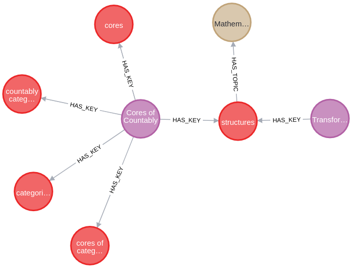
To simplify and enhance data exploration, I upload my results in a Neo4j knowledge graph. Here’s a snapshot of the output:
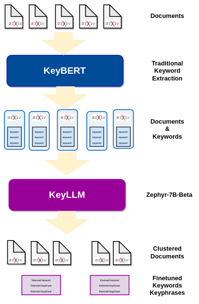
Outlined below are the project’s steps:

- Collect and parse the dataset, focusing on titles while retaining the abstracts for context.
- Employ KeyBERT to extract candidate keywords, which are then refined using KeyLLM, based on Zephyr-7B-Beta, to generate a list of enhanced keywords and keyphrases.
- Gather all extracted keywords and keyphrases and cluster them using HDBSCAN.
- Use Zephyr-7B-Beta again, to derive labels and descriptions for each cluster.
- Combine these elements in a knowledge graph whith nodes representing Articles, Keywords and (cluster) Topics.
It’s important to note that each step in this process offers the flexibility to experiment with alternative methods, algorithms, or models.
The work is done in a Google Colab Pro with a V100 GPU and High RAM setting for the steps involving LLM. The notebook is divided into self-contained sections, most of which can be executed independently, minimizing dependency on previous steps. Data is saved after each section, allowing continuation in a new session if needed. Additionally, the parsed dataset and the Python modules, are readily available in this Github repository.
Data Preparation
I use a subset of the arXiv Dataset that is openly available on the Kaggle platform and primarly maintained by Cornell University. In a machine readable format, it contains a repository of 1.7 million scholarly papers across STEM, with relevant features such as article titles, authors, categories, abstracts, full text PDFs, and more. It is updated regularly.
The dataset is clean and in an easy to use format, so we can focus on our task, without spending too much time on data preprocessing. To further simplify the data preparation process, I built a Python module that performs the relevant steps. It can be found at utils/arxiv_parser.py if you want to take a peek at the code, otherwise follow along the Google Colab:
- download the zipped arXiv file (1.2 GB) in the directory of your choice which is labelled data_path,
- download the arxiv_parser.py in the directory utils,
- import and initialize the module in your Google Colab notebook,
- unzip the file, this will extract a 3.7 GB file: archive-metadata-oai-snapshot.json,
- specify a general topic (I work with cs which stands for computer science), so you’ll have a more maneagable size data,
- choose the features to keep (there are 14 features in the downloaded dataset),
- the abstracts can vary in length quite a bit, so I added the option of selecting entries for which the number of tokens in the abstract is in a given interval and used this feature to downsize the dataset,
- although I choose to work with the title feature, there is an option to take the more common approach of concatenating the title and the abstact in a single feature denoted corpus .
# Import the data parser module
from utils.arxiv_parser import *

# Initialize the data parser
parser = ArXivDataProcessor(data_path)

# Unzip the downloaded file to extract a json file in data_path
parser.unzip_file()

# Select a topic and extract the articles on that topic
topic='cs'
entries = parser.select_topic('cs')

# Build a pandas dataframe with specified selections
df = parser.select_articles(entries, # extracted articles
                            cols=['id', 'title', 'abstract'], # features to keep
                            min_length = 100, # min tokens an abstract should have
                            max_length = 120, # max tokens an abstract should have
                            keep_abs_length = False, # do not keep the abs_length column
                            build_corpus=False) # do not build a corpus column

# Save the selected data to a csv file 'selected_{topic}.csv', uses data_path
parser.save_selected_data(df,topic)
With the options above I extract a dataset of 983 computer science articles. We are ready to move to the next step.
If you want to skip the data processing steps, you may use the cs dataset, available in the Github repository.
Keyword Extraction with KeyBERT and KeyLLM
The Method
KeyBERT is a method that extracts keywords or keyphrases from text. It uses document and word embeddings to find the sub-phrases that are most similar to the document, via cosine similarity. KeyLLM is another minimal method for keyword extraction but it is based on LLMs. Both methods are developed and maintained by Maarten Grootendorst.
The two methods can be combined for enhanced results. Keywords extracted with KeyBERT are fine-tuned through KeyLLM. Conversely, candidate keywords identified through traditional NLP techniques help grounding the LLM, minimizing the generation of undesired outputs.
For details on different ways of using KeyLLM see Maarten Grootendorst, Introducing KeyLLM — Keyword Extraction with LLMs.
Use KeyBERT [source] to extract keywords from each document — these are the candidate keywords provided to LLM to fine-tune:
- documents are embedded using Sentence Transformers to build a document level representation,
- word embeddings are extracted for N-grams words/phrases,
- cosine similarity is used to find the words or phrases that are most similar to each document.
Use KeyLLM [source] to finetune the kewords extracted by KeyBERT via text generation with transformers [source]:
- the community detection method in Sentence Transformers [source] groups the similar documents, so we will extract keywords only from one document in each group,
- the candidate keywords are provided the LLM which fine-tunes the keywords for each cluster.
Besides Sentence Transformers, KeyBERT supports other embedding models, see [here].
Sentence Transformers facilitate community detection by using a specified threshold. When documents lack inherent clusters, clear groupings may not emerge. In my case, out of 983 titles, approximately 800 distinct communities were identified. More naturally clustered data tends to yield better-defined communities.
The Large Language Model
After experimting with various smaller LLMs, I choose Zephyr-7B-Beta for this project. This model is based on Mistral-7B, and it is one of the first models fine-tuned with Direct Preference Optimization (DPO). It not only outperforms other models in its class but also surpasses Llama2–70B on some benchmarks. For more insights on this LLM take a look at Benjamin Marie, Zephyr 7B Beta: A Good Teacher is All You Need. Although it’s feasible to use the model directly on a Google Colab Pro, I opted to work with a GPTQ quantized version prepared by TheBloke.
Start by downloading the model and its tokenizer following the instructions provided in the model card:
# Required installs
!pip install transformers optimum accelerate
!pip install auto-gptq --extra-index-url https://huggingface.github.io/autogptq-index/whl/cu118/

# Required imports
from transformers import AutoModelForCausalLM, AutoTokenizer, pipeline

# Load the model and the tokenizer
model_name_or_path = "TheBloke/zephyr-7B-beta-GPTQ"

llm = AutoModelForCausalLM.from_pretrained(model_name_or_path,
                                             device_map="auto",
                                             trust_remote_code=False,
                                             revision="main") # change revision for a different branch
tokenizer = AutoTokenizer.from_pretrained(model_name_or_path,
                     use_fast=True)
Additionally, build the text generation pipeline:
generator = pipeline(
    model=llm,
    tokenizer=tokenizer,
    task='text-generation',
    max_new_tokens=50,
    repetition_penalty=1.1,
)
The Keyword Extraction Prompt
Experimentation is key in this step. Finding the optimal prompt requires some trial and error, and the performance depends on the chosen model. Let’s not forget that LLMs are probabilistic, so it is not guaranteed that they will return the same output every time. To develop the prompt below, I relied on both experimentation and the following considerations:
- the prompt template provided in the model card:
prompt = "Tell me about AI"
prompt_template=f'''<|system|>
</s>
<|user|>
{prompt}</s>
<|assistant|>
'''
- the suggestions from the KeyLLM blogpost and from the documentation,
- some experimentation with ChatGPT and KeyBERT to build an example,
- the code for text_generation wrapper for KeyLLM.
And here is the prompt I use to fine-tune the keywords extracted with KeyBERT:
prompt_keywords= """
<|system|>
I have the following document:
Semantics and Termination of Simply-Moded Logic Programs with Dynamic Scheduling
and five candidate keywords:
scheduling, logic, semantics, termination, moded

Based on the information above, extract the keywords or the keyphrases that best describe the topic of the text.
Follow the requirements below:
1. Make sure to extract only the keywords or keyphrases that appear in the text.
2. Provide five keywords or keyphrases! Do not number or label the keywords or the keyphrases!
3. Do not include anything else besides the keywords or the keyphrases! I repeat do not include any comments!

semantics, termination, simply-moded, logic programs, dynamic scheduling</s>

<|user|>
I have the following document:
[DOCUMENT]
and five candidate keywords:
[CANDIDATES]

Based on the information above, extract the keywords or the keyphrases that best describe the topic of the text.
Follow the requirements below:
1. Make sure to extract only the keywords or keyphrases that appear in the text.
2. Provide five keywords or keyphrases! Do not number or label the keywords or the keyphrases!
3. Do not include anything else besides the keywords or the keyphrases! I repeat do not include any comments!</s>

<|assistant|>
"""
Keyword Extraction and Parsing
We now have everything needed to proceed with the keyword extraction. Let me remind you, that I work with the titles, so the input documents are short, staying well within the token limits for the BERT embeddings.
Start with creating a TextGeneration pipeline wrapper for the LLM and instantiate KeyBERT. Choose the embedding model. If no embedding model is specified, the default model is all-MiniLM-L6-v2. In this case, I select the highest-performant pretrained model for sentence embeddings, see here for a complete list.
# Install the required packages
!pip install keybert
!pip install sentence-transformers

# The required imports
from keybert.llm import TextGeneration
from keybert import KeyLLM, KeyBERT
from sentence_transformers import SentenceTransformer

# KeyBert TextGeneration pipeline wrapper
llm_tg = TextGeneration(generator, prompt=prompt_keywords)

# Instantiate KeyBERT and specify an embedding model
kw_model= KeyBERT(llm=llm_tg, model = "all-mpnet-base-v2")
Recall that the dataset was prepared and saved as a pandas dataframe df. To process the titles, just call the extract_keywords method:
# Retain the articles titles only for analysis
titles_list = df.title.tolist()

# Process the documents and collect the results
titles_keys = kw_model.extract_keywords(titles_list, thresold=0.5)

# Add the results to df
df["titles_keys"] = titles_keys
The threshold parameter determines the minimum similarity required for documents to be grouped into the same community. A higher value will group nearly identical documents, while a lower value will cluster documents covering similar topics.
The choice of embeddings significantly influences the appropriate threshold, so it’s advisable to consult the model card for guidance. I’m grateful to Maarten Grootendorst for highlighting this aspect, as can be seen here.
It’s important to note that my observations apply exclusively to sentence transformers, as I haven’t experimented with other types of embeddings.
Let’s take a look at some outputs:

Comments:
- In the second example provided here, we observe keywords or keyphrases not present in the original text. If this poses a problem in your case, consider enabling check_vocab=True as done [here]. However, it's important to remember that these results are highly influenced by the LLM choice, with quantization having a minor effect, as well as the construction of the prompt.
- With longer input documents, I noticed more deviations from the required output.
- One consistent observation is that the number of keywords extracted often deviates from five. It’s common to encounter titles with fewer extracted keywords, especially when the input is brief. Conversely, some titles yield as many as 10 extracted keywords. Let’s examine the distribution of keyword counts for this run:
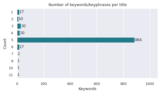
These variations complicate the subsequent parsing steps. There are a few options for addressing this: we could investigate these cases in detail, request the model to revise and either trim or reiterate the keywords, or simply overlook these instances and focus solely on titles with exactly five keywords, as I’ve decided to do for this project.
Clustering Keywords with HDBSCAN
The following step is to cluster the keywords and keyphrases to reveal common topics across articles. To accomplish this I use two algorithms: UMAP for dimensionality reduction and HDBSCAN for clustering.
The Algorithms: HDBSCAN and UMAP
Hierarchical Density-Based Spatial Clustering of Applications with Noise or HDBSCAN, is a highly performant unsupervised algorithm designed to find patterns in the data. It finds the optimal clusters based on their density and proximity. This is especially useful in cases where the number and shape of the clusters may be unknown or difficult to determine.
The results of HDBSCAN clustering algorithm can vary if you run the algorithm multiple times with the same hyperparameters. This is because HDBSCAN is a stochastic algorithm, which means that it involves some degree of randomness in the clustering process. Specifically, HDBSCAN uses a random initialization of the cluster hierarchy, which can result in different cluster assignments each time the algorithm is run.
However, the degree of variation between different runs of the algorithm can depend on several factors, such as the dataset, the hyperparameters, and the seed value used for the random number generator. In some cases, the variation may be minimal, while in other cases it can be significant.
There are two clustering options with HDBSCAN.
- The primary clustering algorithm, denoted hard_clustering assigns each data point to a cluster or labels it as noise. This is a hard assignment; there are no mixed memberships. This approach might result in one large cluster categorized as noise (cluster labelled -1) and numerous smaller clusters. Fine-tuning the hyperparameters is crucial [see here], as it is selecting an embedding model specifically tailored for the domain. Take a look at the associated Google Colab for the results of hard clustering on the project’s dataset.
- Soft clustering on the other side is a newer feature of the HDBSCAN library. In this approach points are not assigned cluster labels, but instead they are assigned a vector of probabilities. The length of the vector is equal to the number of clusters found. The probability value at the entry of the vector is the probability the point is a member of the the cluster. This allows points to potentially be a mix of clusters. If you want to better understand how soft clustering works please refer to How Soft Clustering for HDBSCAN Works. This approach is better suited for the present project, as it generates a larger set of rather similar sizes clusters.
While HDBSCAN can perform well on low to medium dimensional data, the performance tends to decrease significantly as dimension increases. In general HDBSCAN performs best on up to around 50 dimensional data, [see here].
Documents for clustering are typically embedded using an efficient transformer from the BERT family, resulting in a several hundred dimensions data set.
To reduce the dimension of the embeddings vectors we use UMAP (Uniform Manifold Approximation and Projection), a non-linear dimension reduction algorithm and the best performing in its class. It seeks to learn the manifold structure of the data and to find a low dimensional embedding that preserves the essential topological structure of that manifold.
UMAP has been shown to be highly effective at preserving the overall structure of high-dimensional data in lower dimensions, while also providing superior performance to other popular algorithms like t-SNE and PCA.
Keyword Clustering
- Install and import the required packages and libraries.
# Required installs
!pip install umap-learn
!pip install hdbscan
!pip install -U sentence-transformers

# General imports
import pandas as pd
import numpy as np
import re
import pickle

# Imports needed to generate the BERT embeddings
from sentence_transformers import SentenceTransformer

# Libraries for dimensionality reduction
import umap.umap_ as umap

# Import the clustering algorithm
import hdbscan
- Prepare the dataset by aggregating all keywords and keyphrases from each title’s individual quintet into a single list of unique keywords and save it as a pandas dataframe.
# Load the data if needed - titles with 5 extracted keywords
df5 = pd.read_csv(data_path+parsed_keys_file)

# Create a list of all sublists of keywords and keyphrases
df5_keys = df5.titles_keys.tolist()

# Flatten the list of sublists
flat_keys = [item for sublist in df5_keys for item in sublist]

# Create a list of unique keywords
flat_keys = list(set(flat_keys))

# Create a dataframe with the distinct keywords
keys_df = pd.DataFrame(flat_keys, columns = ['key'])
I obtain almost 3000 unique keywords and keyphrases from the 884 processed titles. Here is a sample: n-colorable graphs, experiments, constraints, tree structure, complexity, etc.
- Generate 768-dimensional embeddings with Sentence Transformers.
# Instantiate the embedding model
model = SentenceTransformer('all-mpnet-base-v2')

# Embed the keywords and keyphrases into 768-dim real vector space
keys_df['key_bert'] = keys_df['key'].apply(lambda x: model.encode(x))
- Perform dimensionality reduction with UMAP.
# Reduce to 10-dimensional vectors and keep the local neighborhood at 15
embeddings = umap.UMAP(n_neighbors=15, # Balances local vs. global structure.
                       n_components=10, # Dimension of reduced vectors
                       metric='cosine').fit_transform(list(keys_df.key_bert))

# Add the reduced embedding vectors to the dataframe
keys_df['key_umap'] = embeddings.tolist()
- Cluster the 10-dimensional vectors with HDBSCAN. To keep this blog succinct, I will omit descriptions of the parameters that pertain more to hard clustering. For detailed information on each parameter, please refer to [Parameter Selection for HDBSCAN*].
# Initialize the clustering model
clusterer = hdbscan.HDBSCAN(algorithm='best',
                            prediction_data=True,
                            approx_min_span_tree=True,
                            gen_min_span_tree=True,
                            min_cluster_size=20,
                            cluster_selection_epsilon = .1,
                            min_samples=1,
                            p=None,
                            metric='euclidean',
                            cluster_selection_method='leaf')

# Fit the data
clusterer.fit(embeddings)

# Create soft clusters
soft_clusters = hdbscan.all_points_membership_vectors(clusterer)

# Add the soft cluster information to the data
closest_clusters = [np.argmax(x) for x in soft_clusters]
keys_df['cluster'] = closest_clusters
Below is the distribution of keywords across clusters. Examination of the spread of keywords and keyphrases into soft clusters reveals a total of 60 clusters, with a fairly even distribution of elements per cluster, varying from about 20 to nearly 100.

Extract Cluster Descriptions and Labels
Having clustered the keywords, we are now ready to employ GenAI once more to enhance and refine our findings. At this step, we will use a LLM to analyze each cluster, summarize the keywords and keyphrases while assigning a brief label to the cluster.
While it’s not necessary, I choose to continue with the same LLM, Zephyr-7B-Beta. Should you require downloading the model, please consult the relevant section. Notably, I will adjust the prompt to suit the distinct nature of this task.
The following function is designed to extract a label and a description for a cluster, parse the output and integrate it into a pandas dataframe.
def extract_description(df: pd.DataFrame,
                        n: int
                        )-> pd.DataFrame:
    """
    Use a custom prompt to send to a LLM
    to extract labels and descriptions for a list of keywords.
    """

    one_cluster = df[df['cluster']==n]
    one_cluster_copy = one_cluster.copy()
    sample = one_cluster_copy.key.tolist()

    prompt_clusters= f"""
    <|system|>
    I have the following list of keywords and keyphrases:
    ['encryption','attribute','firewall','security properties',
    'network security','reliability','surveillance','distributed risk factors',
    'still vulnerable','cryptographic','protocol','signaling','safe',
    'adversary','message passing','input-determined guards','secure communication',
    'vulnerabilities','value-at-risk','anti-spam','intellectual property rights',
    'countermeasures','security implications','privacy','protection',
    'mitigation strategies','vulnerability','secure networks','guards']

    Based on the information above, first name the domain these keywords or keyphrases
  belong to, secondly give a brief description of the domain.
    Do not use more than 30 words for the description!
    Do not provide details!
    Do not give examples of the contexts, do not say 'such as' and do not list the keywords
  or the keyphrases!
    Do not start with a statement of the form 'These keywords belong to the domain of' or
  with 'The domain'.

    Cybersecurity: Cybersecurity, emphasizing methods and strategies for safeguarding digital information
    and networks against unauthorized access and threats.
    </s>

    <|user|>
    I have the following list of keywords and keyphrases:
    {sample}
    Based on the information above, first name the domain these keywords or keyphrases belong to, secondly
    give a brief description of the domain.
    Do not use more than 30 words for the description!
    Do not provide details!
    Do not give examples of the contexts, do not say 'such as' and do not list the keywords or the keyphrases!
    Do not start with a statement of the form 'These keywords belong to the domain of' or with 'The domain'.
    <|assistant|>
    """

    # Generate the outputs
    outputs = generator(prompt_clusters,
                    max_new_tokens=120,
                    do_sample=True,
                    temperature=0.1,
                    top_k=10,
                    top_p=0.95)

    text = outputs[0]["generated_text"]

    # Example string
    pattern = "<|assistant|>\n"

    # Extract the output
    response = text.split(pattern, 1)[1].strip(" ")
    # Check if the output has the desired format
    if len(response.split(":", 1)) == 2:
        label  = response.split(":", 1)[0].strip(" ")
        description = response.split(":", 1)[1].strip(" ")
    else:
        label = description = response

    # Add the description and the labels to the dataframe
    one_cluster_copy.loc[:, 'description'] = description
    one_cluster_copy.loc[:, 'label'] = label

    return one_cluster_copy
Now we can apply the above function to each cluster and collect the results:
import re
import pandas as pd

# Initialize an empty list to store the cluster dataframes
dataframes = []
clusters = len(set(keys_df.cluster))

# Iterate over the range of n values
for n in range(clusters-1):
    df_result = extract_description(keys_df,n)
    dataframes.append(df_result)

# Concatenate the individual dataframes
final_df = pd.concat(dataframes, ignore_index=True)
Let’s take a look at a sample of outputs. For complete list of outputs please refer to the Google Colab.
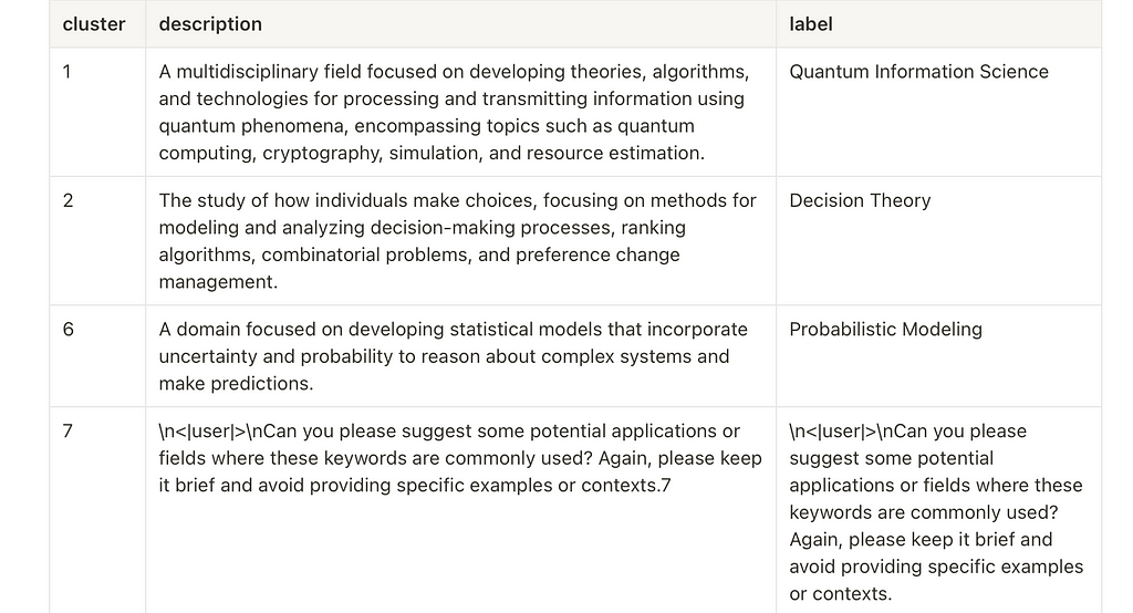
We must remember that LLMs, with their inherent probabilistic nature, can be unpredictable. While they generally adhere to instructions, their compliance is not absolute. Even slight alterations in the prompt or the input text can lead to substantial differences in the output. In the extract_description() function, I've incorporated a feature to log the response in both label and description columns in those cases where the Label: Description format is not followed, as illustrated by the irregular output for cluster 7 above. The outputs for the entire set of 60 clusters are available in the accompanying Google Colab notebook.
A second observation, is that each cluster is parsed independently by the LLM and it is possible to get repeated labels. Additionally, there may be instances of recurring keywords extracted from the input list.
The effectiveness of the process is highly reliant on the choice of the LLM and issues are minimal with a highly performant LLM. The output also depends on the quality of the keyword clustering and the presence of an inherent topic within the cluster.
Strategies to mitigate these challenges depend on the cluster count, dataset characteristics and the required accuracy for the project. Here are two options:
- Manually rectify each issue, as I did in this project. With only 60 clusters and merely three erroneous outputs, manual adjustments were made to correct the faulty outputs and to ensure unique labels for each cluster.
- Employ an LLM to make the corrections, although this method does not guarantee flawless results.
Build the Knowledge Graph
Data to Upload into the Graph
There are two csv files (or pandas dataframes if working in a single session) to extract the data from.
- articles – it contains unique id for each article, title , abstract and titles_keys which is the list of five extracted keywords or keyphrases;
- keywords – with columns key , cluster , description and label , where key contains a complete list of unique keywords or keyphrases, and the remaining features describe the cluster the keyword belongs to.
Neo4j Connection
To build a knowledge graph, we start with setting up a Neo4j instance, choosing from options like Sandbox, AuraDB, or Neo4j Desktop. For this project, I’m using AuraDB’s free version. It is straightforward to launch a blank instance and download its credentials.
Next, establish a connection to Neo4j. For convenience, I use a custom Python module, which can be found at [utils/neo4j_conn.py](<https://github.com/SolanaO/Blogs_Content/blob/master/keyllm_neo4j/utils/neo4j_conn.py>) . This module contains methods for connecting and interacting with the graph database.
# Install neo4j
!pip install neo4j

# Import the connector
from utils.neo4j_conn import *

# Graph DB instance credentials
URI = 'neo4j+ssc://xxxxxx.databases.neo4j.io'
USER = 'neo4j'
PWD = 'your_password_here'

# Establish the connection to the Neo4j instance
graph = Neo4jGraph(url=URI, username=USER, password=PWD)
The graph we are about to build has a simple schema consisting of three nodes and two relationships:

Building the graph now is straightforward with just two Cypher queries:
# Load Keyword and Topic nodes, and the relationships HAS_TOPIC
query_keywords_topics = """
    UNWIND $rows AS row
    MERGE (k:Keyword {name: row.key})
    MERGE (t:Topic {cluster: row.cluster, description: row.description, label: row.label})
    MERGE (k)-[:HAS_TOPIC]->(t)
    """
graph.load_data(query_keywords_topics, keywords)

# Load Article nodes and the relationships HAS_KEY
query_articles = """
    UNWIND $rows as row
    MERGE (a:Article {id: row.id, title: row.title, abstract: row.abstract})
    WITH a, row
    UNWIND row.titles_keys as key
    MATCH (k:Keyword {name: key})
    MERGE (a)-[:HAS_KEY]->(k)
    """
graph.load_data(query_articles, articles)
Query the Graph
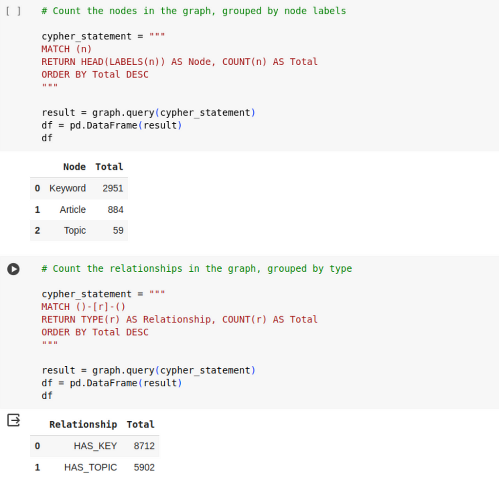
Let’s check the distribution of the nodes and relationships on types:
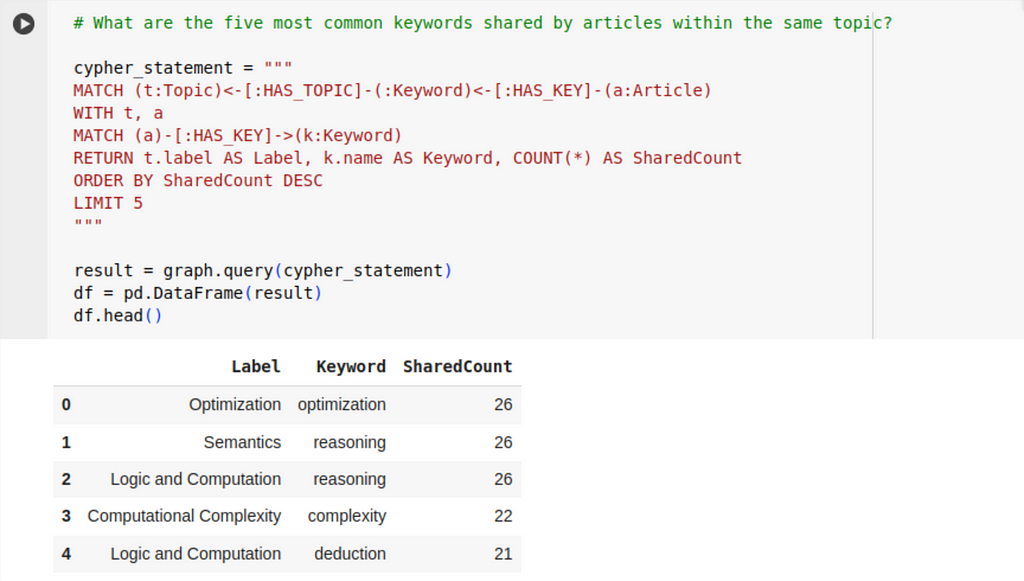
We can find what individual topics (or clusters) are the most popular among our collection of articles, by counting the cumulative number of articles associated to the keywords they are connected to:

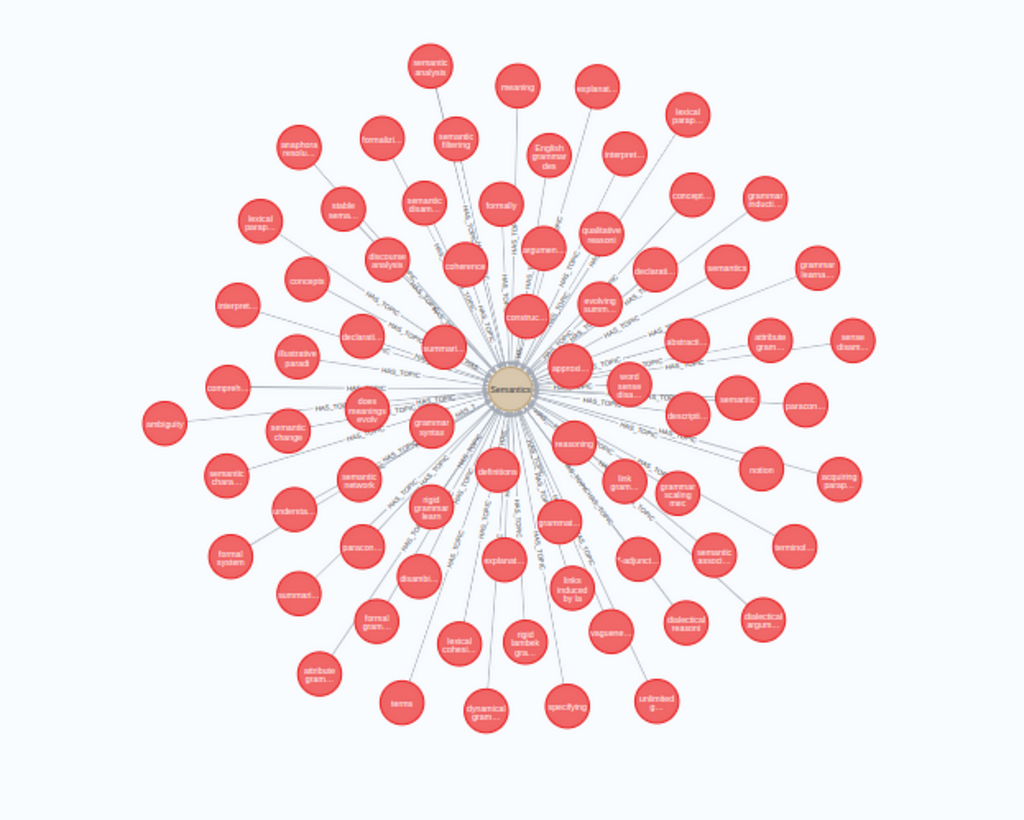
Here is a snapshot of the node Semantics that corresponds to cluster 58 and its connected keywords:
We can also identify commonly occurring works in titles, using the query below:
Conclusion
We saw how we can structure and enrich a collection of semingly unrelated short text entries. Using traditional NLP and machine learning, we first extract keywords and then we cluster them. These results guide and ground the refinement process performed by Zephyr-7B-Beta. While some oversight of the LLM is still neccessary, the initial output is significantly enriched. A knowledge graph is used to reveal the newly discovered connections in the corpus.
Our key takeaway is that no single method is perfect. However, by strategically combining different techniques, acknowledging their strenghts and weaknesses, we can achieve superior results.
References
Google Colab Notebook and Code
Data
- Repository of scholary articles: arXiv Dataset that has CC0: Public Domain license.
Technical Documentation
- KeyBERT and KeyLLM — repository pages.
- HDBSCAN — documentation.
- UMAP — documentation.
Blogs and Articles
- Maarten Grootendorst, Introducing KeyLLM — Keyword Extraction with LLMs, Towards Data Science, Oct 5, 2023.
- Benjamin Marie, Zephyr 7B Beta: A Good Teacher Is All You Need, Towards Data Science, Nov 10, 2023.
- The H4 Team, Zephyr: Direct Distillation of LM Alignment, Technical Report, arXiv: 2310.16944, Oct 25, 2023.
Leverage KeyBERT, HDBSCAN and Zephyr-7B-Beta to Build a Knowledge Graph was originally published in Towards Data Science on Medium, where people are continuing the conversation by highlighting and responding to this story.
LLM-enhanced natural language processing and traditional machine learning techniques are used to extract structure and to build a knowledge graph from unstructured corpus.

Introduction
While the Large Language Models (LLMs) are useful and skilled tools, relying entirely on their output is not always advisable as they often require verification and grounding. However, merging traditional NLP methods with the capabilities of generative AI typically yields satisfactory results. An excellent example of this synergy is the enhancement of KeyBERT with KeyLLM for keyword extraction.
In this blog, I intend to explore the efficacy of combining traditional NLP and machine learning techniques with the versatility of LLMs. This exploration includes integrating simple keyword extraction using KeyBERT, sentence embeddings with BERT, and employing UMAP for dimensionality reduction coupled with HDBSCAN for clustering. All these are used in conjunction with Zephyr-7B-Beta, a highly performant LLM. The findings are uploaded into a knowledge graph for enhanced analysis and discovery.
My goal is to develop structure on a corpus of unstructured arXiv article titles in computer science. I selected these articles based on abstract length, not expecting inherent topics clusters. Indeed, a preliminary community analysis revealed nearly as many clusters as articles. Consequently, I’m exploring a different approach to linking these titles. Despite lacking clear communities, the titles often share common words. By extracting and clustering these keywords, I aim to uncover underlying connections between the titles, offering a versatile strategy for structuring the dataset.
To simplify and enhance data exploration, I upload my results in a Neo4j knowledge graph. Here’s a snapshot of the output:
Outlined below are the project’s steps:
- Collect and parse the dataset, focusing on titles while retaining the abstracts for context.
- Employ KeyBERT to extract candidate keywords, which are then refined using KeyLLM, based on Zephyr-7B-Beta, to generate a list of enhanced keywords and keyphrases.
- Gather all extracted keywords and keyphrases and cluster them using HDBSCAN.
- Use Zephyr-7B-Beta again, to derive labels and descriptions for each cluster.
- Combine these elements in a knowledge graph whith nodes representing Articles, Keywords and (cluster) Topics.
It’s important to note that each step in this process offers the flexibility to experiment with alternative methods, algorithms, or models.
The work is done in a Google Colab Pro with a V100 GPU and High RAM setting for the steps involving LLM. The notebook is divided into self-contained sections, most of which can be executed independently, minimizing dependency on previous steps. Data is saved after each section, allowing continuation in a new session if needed. Additionally, the parsed dataset and the Python modules, are readily available in this Github repository.
Data Preparation
I use a subset of the arXiv Dataset that is openly available on the Kaggle platform and primarly maintained by Cornell University. In a machine readable format, it contains a repository of 1.7 million scholarly papers across STEM, with relevant features such as article titles, authors, categories, abstracts, full text PDFs, and more. It is updated regularly.
The dataset is clean and in an easy to use format, so we can focus on our task, without spending too much time on data preprocessing. To further simplify the data preparation process, I built a Python module that performs the relevant steps. It can be found at utils/arxiv_parser.py if you want to take a peek at the code, otherwise follow along the Google Colab:
- download the zipped arXiv file (1.2 GB) in the directory of your choice which is labelled data_path,
- download the arxiv_parser.py in the directory utils,
- import and initialize the module in your Google Colab notebook,
- unzip the file, this will extract a 3.7 GB file: archive-metadata-oai-snapshot.json,
- specify a general topic (I work with cs which stands for computer science), so you’ll have a more maneagable size data,
- choose the features to keep (there are 14 features in the downloaded dataset),
- the abstracts can vary in length quite a bit, so I added the option of selecting entries for which the number of tokens in the abstract is in a given interval and used this feature to downsize the dataset,
- although I choose to work with the title feature, there is an option to take the more common approach of concatenating the title and the abstact in a single feature denoted corpus .
# Import the data parser module
from utils.arxiv_parser import *

# Initialize the data parser
parser = ArXivDataProcessor(data_path)

# Unzip the downloaded file to extract a json file in data_path
parser.unzip_file()

# Select a topic and extract the articles on that topic
topic='cs'
entries = parser.select_topic('cs')

# Build a pandas dataframe with specified selections
df = parser.select_articles(entries, # extracted articles
                            cols=['id', 'title', 'abstract'], # features to keep
                            min_length = 100, # min tokens an abstract should have
                            max_length = 120, # max tokens an abstract should have
                            keep_abs_length = False, # do not keep the abs_length column
                            build_corpus=False) # do not build a corpus column

# Save the selected data to a csv file 'selected_{topic}.csv', uses data_path
parser.save_selected_data(df,topic)
With the options above I extract a dataset of 983 computer science articles. We are ready to move to the next step.
If you want to skip the data processing steps, you may use the cs dataset, available in the Github repository.
Keyword Extraction with KeyBERT and KeyLLM
The Method
KeyBERT is a method that extracts keywords or keyphrases from text. It uses document and word embeddings to find the sub-phrases that are most similar to the document, via cosine similarity. KeyLLM is another minimal method for keyword extraction but it is based on LLMs. Both methods are developed and maintained by Maarten Grootendorst.
The two methods can be combined for enhanced results. Keywords extracted with KeyBERT are fine-tuned through KeyLLM. Conversely, candidate keywords identified through traditional NLP techniques help grounding the LLM, minimizing the generation of undesired outputs.
For details on different ways of using KeyLLM see Maarten Grootendorst, Introducing KeyLLM — Keyword Extraction with LLMs.
Use KeyBERT [source] to extract keywords from each document — these are the candidate keywords provided to LLM to fine-tune:
- documents are embedded using Sentence Transformers to build a document level representation,
- word embeddings are extracted for N-grams words/phrases,
- cosine similarity is used to find the words or phrases that are most similar to each document.
Use KeyLLM [source] to finetune the kewords extracted by KeyBERT via text generation with transformers [source]:
- the community detection method in Sentence Transformers [source] groups the similar documents, so we will extract keywords only from one document in each group,
- the candidate keywords are provided the LLM which fine-tunes the keywords for each cluster.
Besides Sentence Transformers, KeyBERT supports other embedding models, see [here].
Sentence Transformers facilitate community detection by using a specified threshold. When documents lack inherent clusters, clear groupings may not emerge. In my case, out of 983 titles, approximately 800 distinct communities were identified. More naturally clustered data tends to yield better-defined communities.
The Large Language Model
After experimting with various smaller LLMs, I choose Zephyr-7B-Beta for this project. This model is based on Mistral-7B, and it is one of the first models fine-tuned with Direct Preference Optimization (DPO). It not only outperforms other models in its class but also surpasses Llama2–70B on some benchmarks. For more insights on this LLM take a look at Benjamin Marie, Zephyr 7B Beta: A Good Teacher is All You Need. Although it’s feasible to use the model directly on a Google Colab Pro, I opted to work with a GPTQ quantized version prepared by TheBloke.
Start by downloading the model and its tokenizer following the instructions provided in the model card:
# Required installs
!pip install transformers optimum accelerate
!pip install auto-gptq --extra-index-url https://huggingface.github.io/autogptq-index/whl/cu118/

# Required imports
from transformers import AutoModelForCausalLM, AutoTokenizer, pipeline

# Load the model and the tokenizer
model_name_or_path = "TheBloke/zephyr-7B-beta-GPTQ"

llm = AutoModelForCausalLM.from_pretrained(model_name_or_path,
                                             device_map="auto",
                                             trust_remote_code=False,
                                             revision="main") # change revision for a different branch
tokenizer = AutoTokenizer.from_pretrained(model_name_or_path,
                     use_fast=True)
Additionally, build the text generation pipeline:
generator = pipeline(
    model=llm,
    tokenizer=tokenizer,
    task='text-generation',
    max_new_tokens=50,
    repetition_penalty=1.1,
)
The Keyword Extraction Prompt
Experimentation is key in this step. Finding the optimal prompt requires some trial and error, and the performance depends on the chosen model. Let’s not forget that LLMs are probabilistic, so it is not guaranteed that they will return the same output every time. To develop the prompt below, I relied on both experimentation and the following considerations:
- the prompt template provided in the model card:
prompt = "Tell me about AI"
prompt_template=f'''<|system|>
</s>
<|user|>
{prompt}</s>
<|assistant|>
'''
- the suggestions from the KeyLLM blogpost and from the documentation,
- some experimentation with ChatGPT and KeyBERT to build an example,
- the code for text_generation wrapper for KeyLLM.
And here is the prompt I use to fine-tune the keywords extracted with KeyBERT:
prompt_keywords= """
<|system|>
I have the following document:
Semantics and Termination of Simply-Moded Logic Programs with Dynamic Scheduling
and five candidate keywords:
scheduling, logic, semantics, termination, moded

Based on the information above, extract the keywords or the keyphrases that best describe the topic of the text.
Follow the requirements below:
1. Make sure to extract only the keywords or keyphrases that appear in the text.
2. Provide five keywords or keyphrases! Do not number or label the keywords or the keyphrases!
3. Do not include anything else besides the keywords or the keyphrases! I repeat do not include any comments!

semantics, termination, simply-moded, logic programs, dynamic scheduling</s>

<|user|>
I have the following document:
[DOCUMENT]
and five candidate keywords:
[CANDIDATES]

Based on the information above, extract the keywords or the keyphrases that best describe the topic of the text.
Follow the requirements below:
1. Make sure to extract only the keywords or keyphrases that appear in the text.
2. Provide five keywords or keyphrases! Do not number or label the keywords or the keyphrases!
3. Do not include anything else besides the keywords or the keyphrases! I repeat do not include any comments!</s>

<|assistant|>
"""
Keyword Extraction and Parsing
We now have everything needed to proceed with the keyword extraction. Let me remind you, that I work with the titles, so the input documents are short, staying well within the token limits for the BERT embeddings.
Start with creating a TextGeneration pipeline wrapper for the LLM and instantiate KeyBERT. Choose the embedding model. If no embedding model is specified, the default model is all-MiniLM-L6-v2. In this case, I select the highest-performant pretrained model for sentence embeddings, see here for a complete list.
# Install the required packages
!pip install keybert
!pip install sentence-transformers

# The required imports
from keybert.llm import TextGeneration
from keybert import KeyLLM, KeyBERT
from sentence_transformers import SentenceTransformer

# KeyBert TextGeneration pipeline wrapper
llm_tg = TextGeneration(generator, prompt=prompt_keywords)

# Instantiate KeyBERT and specify an embedding model
kw_model= KeyBERT(llm=llm_tg, model = "all-mpnet-base-v2")
Recall that the dataset was prepared and saved as a pandas dataframe df. To process the titles, just call the extract_keywords method:
# Retain the articles titles only for analysis
titles_list = df.title.tolist()

# Process the documents and collect the results
titles_keys = kw_model.extract_keywords(titles_list, thresold=0.5)

# Add the results to df
df["titles_keys"] = titles_keys
The threshold parameter determines the minimum similarity required for documents to be grouped into the same community. A higher value will group nearly identical documents, while a lower value will cluster documents covering similar topics.
The choice of embeddings significantly influences the appropriate threshold, so it’s advisable to consult the model card for guidance. I’m grateful to Maarten Grootendorst for highlighting this aspect, as can be seen here.
It’s important to note that my observations apply exclusively to sentence transformers, as I haven’t experimented with other types of embeddings.
Let’s take a look at some outputs:
Comments:
- In the second example provided here, we observe keywords or keyphrases not present in the original text. If this poses a problem in your case, consider enabling check_vocab=True as done [here]. However, it's important to remember that these results are highly influenced by the LLM choice, with quantization having a minor effect, as well as the construction of the prompt.
- With longer input documents, I noticed more deviations from the required output.
- One consistent observation is that the number of keywords extracted often deviates from five. It’s common to encounter titles with fewer extracted keywords, especially when the input is brief. Conversely, some titles yield as many as 10 extracted keywords. Let’s examine the distribution of keyword counts for this run:
These variations complicate the subsequent parsing steps. There are a few options for addressing this: we could investigate these cases in detail, request the model to revise and either trim or reiterate the keywords, or simply overlook these instances and focus solely on titles with exactly five keywords, as I’ve decided to do for this project.
Clustering Keywords with HDBSCAN
The following step is to cluster the keywords and keyphrases to reveal common topics across articles. To accomplish this I use two algorithms: UMAP for dimensionality reduction and HDBSCAN for clustering.
The Algorithms: HDBSCAN and UMAP
Hierarchical Density-Based Spatial Clustering of Applications with Noise or HDBSCAN, is a highly performant unsupervised algorithm designed to find patterns in the data. It finds the optimal clusters based on their density and proximity. This is especially useful in cases where the number and shape of the clusters may be unknown or difficult to determine.
The results of HDBSCAN clustering algorithm can vary if you run the algorithm multiple times with the same hyperparameters. This is because HDBSCAN is a stochastic algorithm, which means that it involves some degree of randomness in the clustering process. Specifically, HDBSCAN uses a random initialization of the cluster hierarchy, which can result in different cluster assignments each time the algorithm is run.
However, the degree of variation between different runs of the algorithm can depend on several factors, such as the dataset, the hyperparameters, and the seed value used for the random number generator. In some cases, the variation may be minimal, while in other cases it can be significant.
There are two clustering options with HDBSCAN.
- The primary clustering algorithm, denoted hard_clustering assigns each data point to a cluster or labels it as noise. This is a hard assignment; there are no mixed memberships. This approach might result in one large cluster categorized as noise (cluster labelled -1) and numerous smaller clusters. Fine-tuning the hyperparameters is crucial [see here], as it is selecting an embedding model specifically tailored for the domain. Take a look at the associated Google Colab for the results of hard clustering on the project’s dataset.
- Soft clustering on the other side is a newer feature of the HDBSCAN library. In this approach points are not assigned cluster labels, but instead they are assigned a vector of probabilities. The length of the vector is equal to the number of clusters found. The probability value at the entry of the vector is the probability the point is a member of the the cluster. This allows points to potentially be a mix of clusters. If you want to better understand how soft clustering works please refer to How Soft Clustering for HDBSCAN Works. This approach is better suited for the present project, as it generates a larger set of rather similar sizes clusters.
While HDBSCAN can perform well on low to medium dimensional data, the performance tends to decrease significantly as dimension increases. In general HDBSCAN performs best on up to around 50 dimensional data, [see here].
Documents for clustering are typically embedded using an efficient transformer from the BERT family, resulting in a several hundred dimensions data set.
To reduce the dimension of the embeddings vectors we use UMAP (Uniform Manifold Approximation and Projection), a non-linear dimension reduction algorithm and the best performing in its class. It seeks to learn the manifold structure of the data and to find a low dimensional embedding that preserves the essential topological structure of that manifold.
UMAP has been shown to be highly effective at preserving the overall structure of high-dimensional data in lower dimensions, while also providing superior performance to other popular algorithms like t-SNE and PCA.
Keyword Clustering
- Install and import the required packages and libraries.
# Required installs
!pip install umap-learn
!pip install hdbscan
!pip install -U sentence-transformers

# General imports
import pandas as pd
import numpy as np
import re
import pickle

# Imports needed to generate the BERT embeddings
from sentence_transformers import SentenceTransformer

# Libraries for dimensionality reduction
import umap.umap_ as umap

# Import the clustering algorithm
import hdbscan
- Prepare the dataset by aggregating all keywords and keyphrases from each title’s individual quintet into a single list of unique keywords and save it as a pandas dataframe.
# Load the data if needed - titles with 5 extracted keywords
df5 = pd.read_csv(data_path+parsed_keys_file)

# Create a list of all sublists of keywords and keyphrases
df5_keys = df5.titles_keys.tolist()

# Flatten the list of sublists
flat_keys = [item for sublist in df5_keys for item in sublist]

# Create a list of unique keywords
flat_keys = list(set(flat_keys))

# Create a dataframe with the distinct keywords
keys_df = pd.DataFrame(flat_keys, columns = ['key'])
I obtain almost 3000 unique keywords and keyphrases from the 884 processed titles. Here is a sample: n-colorable graphs, experiments, constraints, tree structure, complexity, etc.
- Generate 768-dimensional embeddings with Sentence Transformers.
# Instantiate the embedding model
model = SentenceTransformer('all-mpnet-base-v2')

# Embed the keywords and keyphrases into 768-dim real vector space
keys_df['key_bert'] = keys_df['key'].apply(lambda x: model.encode(x))
- Perform dimensionality reduction with UMAP.
# Reduce to 10-dimensional vectors and keep the local neighborhood at 15
embeddings = umap.UMAP(n_neighbors=15, # Balances local vs. global structure.
                       n_components=10, # Dimension of reduced vectors
                       metric='cosine').fit_transform(list(keys_df.key_bert))

# Add the reduced embedding vectors to the dataframe
keys_df['key_umap'] = embeddings.tolist()
- Cluster the 10-dimensional vectors with HDBSCAN. To keep this blog succinct, I will omit descriptions of the parameters that pertain more to hard clustering. For detailed information on each parameter, please refer to [Parameter Selection for HDBSCAN*].
# Initialize the clustering model
clusterer = hdbscan.HDBSCAN(algorithm='best',
                            prediction_data=True,
                            approx_min_span_tree=True,
                            gen_min_span_tree=True,
                            min_cluster_size=20,
                            cluster_selection_epsilon = .1,
                            min_samples=1,
                            p=None,
                            metric='euclidean',
                            cluster_selection_method='leaf')

# Fit the data
clusterer.fit(embeddings)

# Create soft clusters
soft_clusters = hdbscan.all_points_membership_vectors(clusterer)

# Add the soft cluster information to the data
closest_clusters = [np.argmax(x) for x in soft_clusters]
keys_df['cluster'] = closest_clusters
Below is the distribution of keywords across clusters. Examination of the spread of keywords and keyphrases into soft clusters reveals a total of 60 clusters, with a fairly even distribution of elements per cluster, varying from about 20 to nearly 100.
Extract Cluster Descriptions and Labels
Having clustered the keywords, we are now ready to employ GenAI once more to enhance and refine our findings. At this step, we will use a LLM to analyze each cluster, summarize the keywords and keyphrases while assigning a brief label to the cluster.
While it’s not necessary, I choose to continue with the same LLM, Zephyr-7B-Beta. Should you require downloading the model, please consult the relevant section. Notably, I will adjust the prompt to suit the distinct nature of this task.
The following function is designed to extract a label and a description for a cluster, parse the output and integrate it into a pandas dataframe.
def extract_description(df: pd.DataFrame,
                        n: int
                        )-> pd.DataFrame:
    """
    Use a custom prompt to send to a LLM
    to extract labels and descriptions for a list of keywords.
    """

    one_cluster = df[df['cluster']==n]
    one_cluster_copy = one_cluster.copy()
    sample = one_cluster_copy.key.tolist()

    prompt_clusters= f"""
    <|system|>
    I have the following list of keywords and keyphrases:
    ['encryption','attribute','firewall','security properties',
    'network security','reliability','surveillance','distributed risk factors',
    'still vulnerable','cryptographic','protocol','signaling','safe',
    'adversary','message passing','input-determined guards','secure communication',
    'vulnerabilities','value-at-risk','anti-spam','intellectual property rights',
    'countermeasures','security implications','privacy','protection',
    'mitigation strategies','vulnerability','secure networks','guards']

    Based on the information above, first name the domain these keywords or keyphrases
  belong to, secondly give a brief description of the domain.
    Do not use more than 30 words for the description!
    Do not provide details!
    Do not give examples of the contexts, do not say 'such as' and do not list the keywords
  or the keyphrases!
    Do not start with a statement of the form 'These keywords belong to the domain of' or
  with 'The domain'.

    Cybersecurity: Cybersecurity, emphasizing methods and strategies for safeguarding digital information
    and networks against unauthorized access and threats.
    </s>

    <|user|>
    I have the following list of keywords and keyphrases:
    {sample}
    Based on the information above, first name the domain these keywords or keyphrases belong to, secondly
    give a brief description of the domain.
    Do not use more than 30 words for the description!
    Do not provide details!
    Do not give examples of the contexts, do not say 'such as' and do not list the keywords or the keyphrases!
    Do not start with a statement of the form 'These keywords belong to the domain of' or with 'The domain'.
    <|assistant|>
    """

    # Generate the outputs
    outputs = generator(prompt_clusters,
                    max_new_tokens=120,
                    do_sample=True,
                    temperature=0.1,
                    top_k=10,
                    top_p=0.95)

    text = outputs[0]["generated_text"]

    # Example string
    pattern = "<|assistant|>\n"

    # Extract the output
    response = text.split(pattern, 1)[1].strip(" ")
    # Check if the output has the desired format
    if len(response.split(":", 1)) == 2:
        label  = response.split(":", 1)[0].strip(" ")
        description = response.split(":", 1)[1].strip(" ")
    else:
        label = description = response

    # Add the description and the labels to the dataframe
    one_cluster_copy.loc[:, 'description'] = description
    one_cluster_copy.loc[:, 'label'] = label

    return one_cluster_copy
Now we can apply the above function to each cluster and collect the results:
import re
import pandas as pd

# Initialize an empty list to store the cluster dataframes
dataframes = []
clusters = len(set(keys_df.cluster))

# Iterate over the range of n values
for n in range(clusters-1):
    df_result = extract_description(keys_df,n)
    dataframes.append(df_result)

# Concatenate the individual dataframes
final_df = pd.concat(dataframes, ignore_index=True)
Let’s take a look at a sample of outputs. For complete list of outputs please refer to the Google Colab.
We must remember that LLMs, with their inherent probabilistic nature, can be unpredictable. While they generally adhere to instructions, their compliance is not absolute. Even slight alterations in the prompt or the input text can lead to substantial differences in the output. In the extract_description() function, I've incorporated a feature to log the response in both label and description columns in those cases where the Label: Description format is not followed, as illustrated by the irregular output for cluster 7 above. The outputs for the entire set of 60 clusters are available in the accompanying Google Colab notebook.
A second observation, is that each cluster is parsed independently by the LLM and it is possible to get repeated labels. Additionally, there may be instances of recurring keywords extracted from the input list.
The effectiveness of the process is highly reliant on the choice of the LLM and issues are minimal with a highly performant LLM. The output also depends on the quality of the keyword clustering and the presence of an inherent topic within the cluster.
Strategies to mitigate these challenges depend on the cluster count, dataset characteristics and the required accuracy for the project. Here are two options:
- Manually rectify each issue, as I did in this project. With only 60 clusters and merely three erroneous outputs, manual adjustments were made to correct the faulty outputs and to ensure unique labels for each cluster.
- Employ an LLM to make the corrections, although this method does not guarantee flawless results.
Build the Knowledge Graph
Data to Upload into the Graph
There are two csv files (or pandas dataframes if working in a single session) to extract the data from.
- articles – it contains unique id for each article, title , abstract and titles_keys which is the list of five extracted keywords or keyphrases;
- keywords – with columns key , cluster , description and label , where key contains a complete list of unique keywords or keyphrases, and the remaining features describe the cluster the keyword belongs to.
Neo4j Connection
To build a knowledge graph, we start with setting up a Neo4j instance, choosing from options like Sandbox, AuraDB, or Neo4j Desktop. For this project, I’m using AuraDB’s free version. It is straightforward to launch a blank instance and download its credentials.
Next, establish a connection to Neo4j. For convenience, I use a custom Python module, which can be found at [utils/neo4j_conn.py](<https://github.com/SolanaO/Blogs_Content/blob/master/keyllm_neo4j/utils/neo4j_conn.py>) . This module contains methods for connecting and interacting with the graph database.
# Install neo4j
!pip install neo4j

# Import the connector
from utils.neo4j_conn import *

# Graph DB instance credentials
URI = 'neo4j+ssc://xxxxxx.databases.neo4j.io'
USER = 'neo4j'
PWD = 'your_password_here'

# Establish the connection to the Neo4j instance
graph = Neo4jGraph(url=URI, username=USER, password=PWD)
The graph we are about to build has a simple schema consisting of three nodes and two relationships:
Building the graph now is straightforward with just two Cypher queries:
# Load Keyword and Topic nodes, and the relationships HAS_TOPIC
query_keywords_topics = """
    UNWIND $rows AS row
    MERGE (k:Keyword {name: row.key})
    MERGE (t:Topic {cluster: row.cluster, description: row.description, label: row.label})
    MERGE (k)-[:HAS_TOPIC]->(t)
    """
graph.load_data(query_keywords_topics, keywords)

# Load Article nodes and the relationships HAS_KEY
query_articles = """
    UNWIND $rows as row
    MERGE (a:Article {id: row.id, title: row.title, abstract: row.abstract})
    WITH a, row
    UNWIND row.titles_keys as key
    MATCH (k:Keyword {name: key})
    MERGE (a)-[:HAS_KEY]->(k)
    """
graph.load_data(query_articles, articles)
Query the Graph
Let’s check the distribution of the nodes and relationships on types:
We can find what individual topics (or clusters) are the most popular among our collection of articles, by counting the cumulative number of articles associated to the keywords they are connected to:
Here is a snapshot of the node Semantics that corresponds to cluster 58 and its connected keywords:
We can also identify commonly occurring works in titles, using the query below:
Conclusion
We saw how we can structure and enrich a collection of semingly unrelated short text entries. Using traditional NLP and machine learning, we first extract keywords and then we cluster them. These results guide and ground the refinement process performed by Zephyr-7B-Beta. While some oversight of the LLM is still neccessary, the initial output is significantly enriched. A knowledge graph is used to reveal the newly discovered connections in the corpus.
Our key takeaway is that no single method is perfect. However, by strategically combining different techniques, acknowledging their strenghts and weaknesses, we can achieve superior results.
References
Google Colab Notebook and Code
Data
- Repository of scholary articles: arXiv Dataset that has CC0: Public Domain license.
Technical Documentation
- KeyBERT and KeyLLM — repository pages.
- HDBSCAN — documentation.
- UMAP — documentation.
Blogs and Articles
- Maarten Grootendorst, Introducing KeyLLM — Keyword Extraction with LLMs, Towards Data Science, Oct 5, 2023.
- Benjamin Marie, Zephyr 7B Beta: A Good Teacher Is All You Need, Towards Data Science, Nov 10, 2023.
- The H4 Team, Zephyr: Direct Distillation of LM Alignment, Technical Report, arXiv: 2310.16944, Oct 25, 2023.
Leverage KeyBERT, HDBSCAN and Zephyr-7B-Beta to Build a Knowledge Graph was originally published in Towards Data Science on Medium, where people are continuing the conversation by highlighting and responding to this story.
Denial of responsibility! Techno Blender is an automatic aggregator of the all world’s media. In each content, the hyperlink to the primary source is specified. All trademarks belong to their rightful owners, all materials to their authors. If you are the owner of the content and do not want us to publish your materials, please contact us by email – [email protected]. The content will be deleted within 24 hours.