
Machine Learning on a Large Scale | by Pan Cretan | Jun, 2022
A demonstration using binomial and multinomial logistic regression in PySpark
With the release of Spark 3.2.1, that has been locally deployed for this article, PySpark offers a fluent API that resembles the expressivity of scikit-learn but additionally offers the benefits of distributed computing. This article demonstrates the use of the pyspark.ml module for constructing ML pipelines on top of Spark data frames (instead of RDDs with the older pyspark.mllib module). The functionality is exemplified using binomial and multinomial logistic regression that admittedly are not the most advanced machine learning algorithms. Still, their simplicity makes them ideal for demonstrating the PySpark machine learning API. This tutorial may be of interest to readers that are new to machine learning with PySpark and to readers who are more familiar with earlier versions of Spark and in particular of the pyspark.mllib module.
Table of contents
· Setting the scene
· Binomial logistic regression
∘ Preparatory work
∘ First modelling attempt
∘ Assessing model quality
∘ Cross-validation and hyper-parameter tuning
∘ Model interpretation
· Multinomial logistic regression
· Conclusions
We first create a spark session by allocating 8 GiB of memory and four cores
The code above also contains all required pyspark imports for the whole article. When it comes to other packages, we will be using some more imports as the need arises.
We will use the iris dataset obtained from seaborn using df = sns.load_dataset('iris'). This is a famous dataset that contains four continuous features, namely the sepal and petal lengths and widths of 150 iris flowers that belong to three different species: Iris setosa, Iris versicolor and Iris virginica. The dataset does not have null values and all features are reasonably well scaled, but we will return to this later.
Obviously this is a very small dataset that by no means requires distributed computing. However, given that the purpose of this article is to illustrate the PySpark machine learning API, choosing a small dataset is ideal for experimenting, especially when using cross-validation for hyper-parameter tuning as we do in this article. Using a basic machine learning algorithm and a small, reasonably clean dataset does not break new frontiers in data science, but these choices are intentional.
In order to get an idea of how well the classification may work, we plot the pairwise relationships in the dataset using sns.pairplot(df, hue='species') that gives
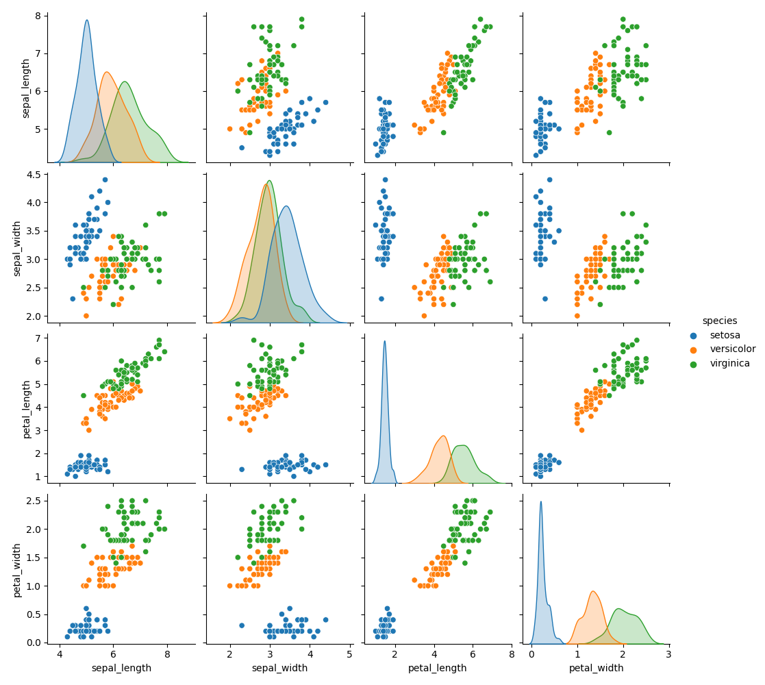
With a cursory look we can see that Iris setosa is likely to be classified correctly, but we expect some difficulty in distinguishing Iris versicolor and Iris virginica.
For simplicity we will use the same dataset for both binomial and multinomial logistic regression. For binary classification we attempt to predict whether the species is Iris virginica vs. not Iris virginica
From this point onwards all operations will take place in PySpark by converting the pandas data frame into a PySpark one
The automatic conversion automatically produced the expected schema.
Preparatory work
PySpark uses transformers and estimators to transform data into machine learning features:
- a transformer is an algorithm which can transform one data frame into another data frame
- an estimator is an algorithm which can be fitted on a data frame to produce a transformer
The above means that a transformer does not depend on the data. A machine learning model is a transformer that takes a data frame with features and produces a data frame that also contains predictions via its.transform() method. On the other hand, an estimator has a.fit() method that accepts a data frame and produces a transformer. A pipeline in PySpark chains multiple transformers and estimators in an ML workflow. Users of scikit-learn will surely feel at home!
Going back to our dataset, we construct the first transformer to pack the four features into a vector
The features column looks like an array but it is a vector. Conveniently, the vector assembler also populates the metadata property of the features column in the schema
and it is possible to retrieve the column names of the original features, although this may be more conveniently done using feature_assembler.getInputCols().
Although the features are more or less scaled, the interpretation of the fitted logistic regression coefficients will be facilitated if we ensure that all features range from 0 to 1. This can be achieved using a min-max scaler estimator
In the code above minMax_scaler_model is a transformer produced by fitting the minMax_scaler estimator to the data. It is convenient to be able to scale all continuous features in one go by using a vector. Incidentally, the pyspark.ml.feature module contains thevector_to_array() and array_to_vector()functions to interconvert vectors and arrays, so estimators like the minMax_scaler can also be used in data transformations beyond machine learning.
In principle, the features_scaled and species columns can now be used to fit a logistic regression model. However, before doing so we will introduce one more concept, the ML pipeline that can be used to orchestrate ML workflows
The results are identical as before, but the code is more succinct. The pipeline is technically an estimator and has a .fit() function that returns a transformer. Behind the scenes, fitting a pipeline calls the .transform() function for transformers and the .fit() function for estimators, in the order they have been introduced in the pipeline stages. In practice, we can build more than one pipeline with different transformers and estimators and experiment with building models to see the effect of our choices.
First modelling attempt
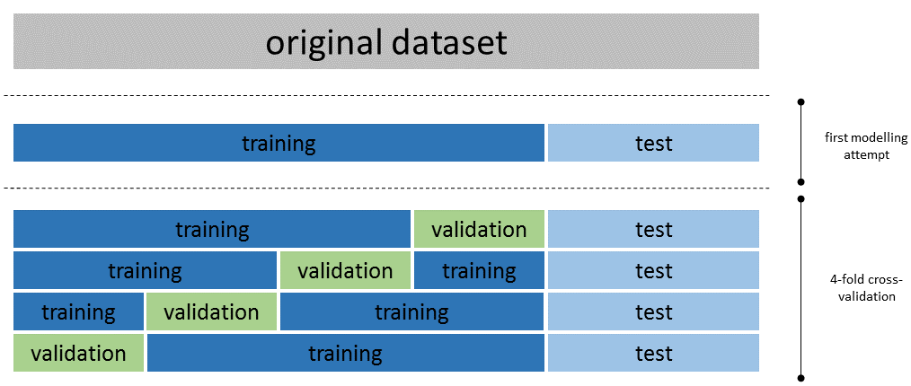
Before tuning the model and assessing its accuracy, it is useful to make a first, crude attempt to see what are the chances of ending up with a reasonable model. For doing so we do not use cross-validation and we only specify the obligatory model parameters leaving all the rest to their defaults.
The first thing to do is to add one more pipeline stage, namely the conversion of the species column from string to numerical using a StringIndexerModel
as this is required later on. Alternatively, we could have used the StringIndexer estimator to create the model by using the data and assign the indices based on the frequency of the species names. We opted against this because we wanted to ensure that Iris virginica is mapped to 1.0 and not Iris virginica to 0.0. We then split the data set into training and test set
We specified the seed as a good practice, although in the Spark world this does not ensure deterministic behaviour due to underlying partitioning of the data. If you are curious about this mind-boggling topic the following experiment can exemplify the issue
You can read more in this article, including ideas on how to avoid this issue, e.g. by caching the whole dataset instead of only the training set (as done below). Storing the training and test sets and reading them again for building the model is another way to ensure deterministic behaviour. Note, that the training dataset should in any case always be cached given that it is used repeatedly when the model is fitted. This is likely the most typical use case for caching in Spark.
The only thing that remains is to fit the model and evaluate its accuracy. For the sake of completeness the whole code is provided so it is easier to follow along
For convenience we converted the predicted numerical values back to labels using pyspark.ml.feature.IndexToString(). Please note that we only used the sepal width and petal width as independent variables. In addition, we only used 20% of the dataset for training. The reason for these strange choices is that this machine learning problem is in fact very easy to tackle and hence we almost always obtain a good model with little effort. By dropping some features and by using a small training set we compute metrics that are not perfect from the outset.
We now have the predictions for the test set and can get a glimpse on how well we did.
Assessing model quality
Perhaps the most common way to obtain an idea about the performance of a binomial classification model is to compute the confusion matrix. In PySpark this is easily done manually with
The confusion matrix can also be easily visualised using an annotated heatmap in seaborn
that produces
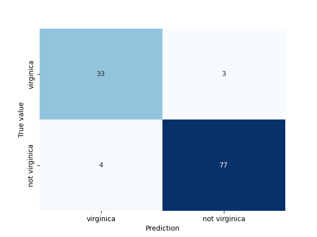
If you try to follow along you may obtain slightly different results due to the different split into training and test sets.
There are many metrics that can be computed, but I list the most important that are also relevant for the ROC curve calculation later on:
- Recall, sensitivity or true positive rate: It reflects the ability of the model to identify the positives and is defined as TP/(TP+FN)
- Precision or positive predictive value: It shows how often a predicted positive is a true positive and is defined as TP/(TP+FP)
- Specificity or true negative rate: It reflects the ability of the model to identify the negatives and is defined as TN/(TN+FP)
- False positive rate: It reflects the probability of a false positive and is defined as FP/(TN+FP) = 1-specificity
These metrics are easy to calculate manually after the confusion matrix has been computed. Alternatively, the PySpark API can also be used for convenience
The receiver operator characteristic (ROC) curve for the test set can be retrieved from metrics.roc but we will also compute it manually using the raw probabilities. We use seaborn to visualise the results of the two approaches
that produces
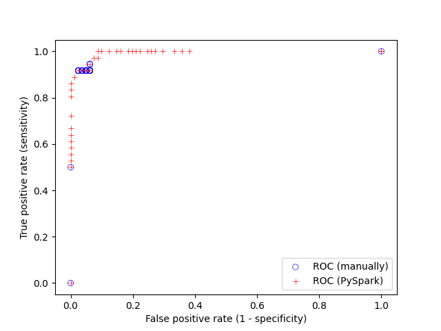
I would not advise to compute the ROC curve manually for several reasons that includes performance worries. However, it is good to be cautious given that the PySpark machine learning API based on data frames is new and the documentation is not yet perfect. Checking that the results make sense is advisable to ensure that the API is used correctly. The PySpark API can also return the precision-recall (PR) curve that is useful when the the classes are very unbalanced. The purpose of the ROC curve is to select the threshold in order to achieve the desired sensitivity and specificity. The threshold can be seen as a parameter of the model, and as with all parameters it should not be calculated on the test set but on the training set, or even better, on the validation set (see next section). The PySpark API provides the ROC and PR curves for the training set curves thought lr_model.summary.roc and lr_model.summary.pr.
The ROC curve is also used in order to compute the area under the ROC curve metric. The ROC curve of a perfect model will approach the top-left corner, whilst a random model will approach the diagonal (True positive rate = False positive rate). The area under the ROC curve ranges between 0. and 1 and can be computed via a BinaryClassificationEvaluator object
The result is impressive, despite the attempt to hamper the model quality. The area under the ROC curve for the training set can be obtained from the model summary lr_model.summary.areaUnderROC. The BinaryClassificationEvaluator object can also be used to compute the area under the PR curve.
Cross-validation and hyper-parameter tuning
The logistic regression model, like most other models, have parameters that can be fine-tuned in order to optimise the model accuracy and robustness. The previous section describes a first modelling attempt that cut many corners. We used the default value for all parameters of the logistic regression model and we simplified model development by splitting the original dataset into two parts only, one for training and one for testing. This is a a good way to start in order to obtain a first idea of what can be achieved. Once we are confident that we are likely to produce a viable model we can use cross-validation to optimise the parameters of the model. This is an expensive operation. First of all, for a given set of model parameters we fit and evaluate the model multiple times (that is known as folds). Secondly, we try many different sets of model parameters. This section gives the complete code for binomial logistic regression using 4-fold cross-validation and serves as an example on how other machine learning models in PySpark can be trained and optimised.
Cross-validation requires three building blocks:
- an estimator (model), that is typically packed in a ML pipeline
- a grid with the hyper-parameters we are trying to tune
- an evaluation metric that is essentially the objective function for the hyper-parameter tuning
In our example we use the earlier set pipeline. We will fine-tune two parameters of the logistic regression model, namely
It may sound strange, but we will also use hyper-parameter tuning for selecting features by adjusting the features passed to the vector assembler. This is a bit far fetched for this example, but I opted for this to show that all parameters of all pipeline stages can in principle be included in the fine-tuning. The number of parameter combinations grows quickly out of hand and in practice run time constraints curb the enthusiasm.
The evaluator used is the area under the ROC curve computed (correctly) over the validation sets averaged over the different folds.
The grid search examined 165 parameter combinations, each of which fitted and evaluated four models. This took ~350 sec despite the fact that the iris dataset is very small compared to the datasets typically handled with Spark. The average area under the ROC curve for each parameter combination can retrieved withcv_model.avgMetrics that shows that several combinations achieved a nearly perfect metric (area under the ROC curve ~=1.). The best model can be retrieved from withcv_model.bestModel (not sure how Spark selects the best model when two sets of parameters perform equally well, but this is less likely to happen in real world use cases).
All the fitted models are stored and can be retrieved with cv_model.subModels[k][i] where k is the fold and i the index of the parameter set in the parameter grid. In our example, the best results were obtained for i=4 and the 4 models corresponding to the four folds can be obtained with [cv_model.subModels[k][4] for k in range(4)]. We should check the distribution of coefficients for the different folds that is an indication of model stability and even fit the whole training set once more using the optimal hyper-parameters. This goes beyond the scope of this article. We will instead use the best model returned with cv_model.bestModel with no further investigations.
Model interpretation
It is perhaps surprising that by using only the sepal and petal widths without regularisation we obtain a very good model. The coefficients and intercept of the linear model can be easily retrieved
and stored in a pandas Series. Conveniently the vector assembler stores the feature names as schema metadata that can be used to set the series index. The features had been min-max scaled that helps with the interpretation. The petal width has roughly 4 times more impact than the sepal width.
This is a special situation: the hyper-parameter tuning happened to only keep two features, whilst no regularisation was necessary. This allows visualising the decision boundary, with the only complexity being the handling of the feature scaling
that produces
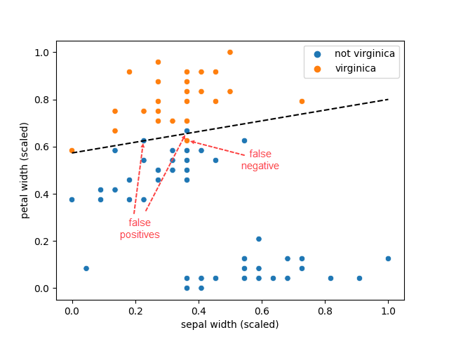
Figure 5 displays the training set (meaning all data points other than the test set) and we can see that there is one false negative and two false positives (one almost on the decision boundary), that is consistent with the confusion matrix for the training set. It all looks good.
PySpark also supports multinomial logistic regression (softmax) and hence it is possible to predict all classes for the iris dataset in one go. We will not cover all details because the article is already quite long. The complete code with the first attempt to fit a multinomial logistic regression model can be found below
Once more we obtain a good model with the first attempt.
A demonstration using binomial and multinomial logistic regression in PySpark
With the release of Spark 3.2.1, that has been locally deployed for this article, PySpark offers a fluent API that resembles the expressivity of scikit-learn but additionally offers the benefits of distributed computing. This article demonstrates the use of the pyspark.ml module for constructing ML pipelines on top of Spark data frames (instead of RDDs with the older pyspark.mllib module). The functionality is exemplified using binomial and multinomial logistic regression that admittedly are not the most advanced machine learning algorithms. Still, their simplicity makes them ideal for demonstrating the PySpark machine learning API. This tutorial may be of interest to readers that are new to machine learning with PySpark and to readers who are more familiar with earlier versions of Spark and in particular of the pyspark.mllib module.
Table of contents
· Setting the scene
· Binomial logistic regression
∘ Preparatory work
∘ First modelling attempt
∘ Assessing model quality
∘ Cross-validation and hyper-parameter tuning
∘ Model interpretation
· Multinomial logistic regression
· Conclusions
We first create a spark session by allocating 8 GiB of memory and four cores
The code above also contains all required pyspark imports for the whole article. When it comes to other packages, we will be using some more imports as the need arises.
We will use the iris dataset obtained from seaborn using df = sns.load_dataset('iris'). This is a famous dataset that contains four continuous features, namely the sepal and petal lengths and widths of 150 iris flowers that belong to three different species: Iris setosa, Iris versicolor and Iris virginica. The dataset does not have null values and all features are reasonably well scaled, but we will return to this later.
Obviously this is a very small dataset that by no means requires distributed computing. However, given that the purpose of this article is to illustrate the PySpark machine learning API, choosing a small dataset is ideal for experimenting, especially when using cross-validation for hyper-parameter tuning as we do in this article. Using a basic machine learning algorithm and a small, reasonably clean dataset does not break new frontiers in data science, but these choices are intentional.
In order to get an idea of how well the classification may work, we plot the pairwise relationships in the dataset using sns.pairplot(df, hue='species') that gives
With a cursory look we can see that Iris setosa is likely to be classified correctly, but we expect some difficulty in distinguishing Iris versicolor and Iris virginica.
For simplicity we will use the same dataset for both binomial and multinomial logistic regression. For binary classification we attempt to predict whether the species is Iris virginica vs. not Iris virginica
From this point onwards all operations will take place in PySpark by converting the pandas data frame into a PySpark one
The automatic conversion automatically produced the expected schema.
Preparatory work
PySpark uses transformers and estimators to transform data into machine learning features:
- a transformer is an algorithm which can transform one data frame into another data frame
- an estimator is an algorithm which can be fitted on a data frame to produce a transformer
The above means that a transformer does not depend on the data. A machine learning model is a transformer that takes a data frame with features and produces a data frame that also contains predictions via its.transform() method. On the other hand, an estimator has a.fit() method that accepts a data frame and produces a transformer. A pipeline in PySpark chains multiple transformers and estimators in an ML workflow. Users of scikit-learn will surely feel at home!
Going back to our dataset, we construct the first transformer to pack the four features into a vector
The features column looks like an array but it is a vector. Conveniently, the vector assembler also populates the metadata property of the features column in the schema
and it is possible to retrieve the column names of the original features, although this may be more conveniently done using feature_assembler.getInputCols().
Although the features are more or less scaled, the interpretation of the fitted logistic regression coefficients will be facilitated if we ensure that all features range from 0 to 1. This can be achieved using a min-max scaler estimator
In the code above minMax_scaler_model is a transformer produced by fitting the minMax_scaler estimator to the data. It is convenient to be able to scale all continuous features in one go by using a vector. Incidentally, the pyspark.ml.feature module contains thevector_to_array() and array_to_vector()functions to interconvert vectors and arrays, so estimators like the minMax_scaler can also be used in data transformations beyond machine learning.
In principle, the features_scaled and species columns can now be used to fit a logistic regression model. However, before doing so we will introduce one more concept, the ML pipeline that can be used to orchestrate ML workflows
The results are identical as before, but the code is more succinct. The pipeline is technically an estimator and has a .fit() function that returns a transformer. Behind the scenes, fitting a pipeline calls the .transform() function for transformers and the .fit() function for estimators, in the order they have been introduced in the pipeline stages. In practice, we can build more than one pipeline with different transformers and estimators and experiment with building models to see the effect of our choices.
First modelling attempt
Before tuning the model and assessing its accuracy, it is useful to make a first, crude attempt to see what are the chances of ending up with a reasonable model. For doing so we do not use cross-validation and we only specify the obligatory model parameters leaving all the rest to their defaults.
The first thing to do is to add one more pipeline stage, namely the conversion of the species column from string to numerical using a StringIndexerModel
as this is required later on. Alternatively, we could have used the StringIndexer estimator to create the model by using the data and assign the indices based on the frequency of the species names. We opted against this because we wanted to ensure that Iris virginica is mapped to 1.0 and not Iris virginica to 0.0. We then split the data set into training and test set
We specified the seed as a good practice, although in the Spark world this does not ensure deterministic behaviour due to underlying partitioning of the data. If you are curious about this mind-boggling topic the following experiment can exemplify the issue
You can read more in this article, including ideas on how to avoid this issue, e.g. by caching the whole dataset instead of only the training set (as done below). Storing the training and test sets and reading them again for building the model is another way to ensure deterministic behaviour. Note, that the training dataset should in any case always be cached given that it is used repeatedly when the model is fitted. This is likely the most typical use case for caching in Spark.
The only thing that remains is to fit the model and evaluate its accuracy. For the sake of completeness the whole code is provided so it is easier to follow along
For convenience we converted the predicted numerical values back to labels using pyspark.ml.feature.IndexToString(). Please note that we only used the sepal width and petal width as independent variables. In addition, we only used 20% of the dataset for training. The reason for these strange choices is that this machine learning problem is in fact very easy to tackle and hence we almost always obtain a good model with little effort. By dropping some features and by using a small training set we compute metrics that are not perfect from the outset.
We now have the predictions for the test set and can get a glimpse on how well we did.
Assessing model quality
Perhaps the most common way to obtain an idea about the performance of a binomial classification model is to compute the confusion matrix. In PySpark this is easily done manually with
The confusion matrix can also be easily visualised using an annotated heatmap in seaborn
that produces
If you try to follow along you may obtain slightly different results due to the different split into training and test sets.
There are many metrics that can be computed, but I list the most important that are also relevant for the ROC curve calculation later on:
- Recall, sensitivity or true positive rate: It reflects the ability of the model to identify the positives and is defined as TP/(TP+FN)
- Precision or positive predictive value: It shows how often a predicted positive is a true positive and is defined as TP/(TP+FP)
- Specificity or true negative rate: It reflects the ability of the model to identify the negatives and is defined as TN/(TN+FP)
- False positive rate: It reflects the probability of a false positive and is defined as FP/(TN+FP) = 1-specificity
These metrics are easy to calculate manually after the confusion matrix has been computed. Alternatively, the PySpark API can also be used for convenience
The receiver operator characteristic (ROC) curve for the test set can be retrieved from metrics.roc but we will also compute it manually using the raw probabilities. We use seaborn to visualise the results of the two approaches
that produces
I would not advise to compute the ROC curve manually for several reasons that includes performance worries. However, it is good to be cautious given that the PySpark machine learning API based on data frames is new and the documentation is not yet perfect. Checking that the results make sense is advisable to ensure that the API is used correctly. The PySpark API can also return the precision-recall (PR) curve that is useful when the the classes are very unbalanced. The purpose of the ROC curve is to select the threshold in order to achieve the desired sensitivity and specificity. The threshold can be seen as a parameter of the model, and as with all parameters it should not be calculated on the test set but on the training set, or even better, on the validation set (see next section). The PySpark API provides the ROC and PR curves for the training set curves thought lr_model.summary.roc and lr_model.summary.pr.
The ROC curve is also used in order to compute the area under the ROC curve metric. The ROC curve of a perfect model will approach the top-left corner, whilst a random model will approach the diagonal (True positive rate = False positive rate). The area under the ROC curve ranges between 0. and 1 and can be computed via a BinaryClassificationEvaluator object
The result is impressive, despite the attempt to hamper the model quality. The area under the ROC curve for the training set can be obtained from the model summary lr_model.summary.areaUnderROC. The BinaryClassificationEvaluator object can also be used to compute the area under the PR curve.
Cross-validation and hyper-parameter tuning
The logistic regression model, like most other models, have parameters that can be fine-tuned in order to optimise the model accuracy and robustness. The previous section describes a first modelling attempt that cut many corners. We used the default value for all parameters of the logistic regression model and we simplified model development by splitting the original dataset into two parts only, one for training and one for testing. This is a a good way to start in order to obtain a first idea of what can be achieved. Once we are confident that we are likely to produce a viable model we can use cross-validation to optimise the parameters of the model. This is an expensive operation. First of all, for a given set of model parameters we fit and evaluate the model multiple times (that is known as folds). Secondly, we try many different sets of model parameters. This section gives the complete code for binomial logistic regression using 4-fold cross-validation and serves as an example on how other machine learning models in PySpark can be trained and optimised.
Cross-validation requires three building blocks:
- an estimator (model), that is typically packed in a ML pipeline
- a grid with the hyper-parameters we are trying to tune
- an evaluation metric that is essentially the objective function for the hyper-parameter tuning
In our example we use the earlier set pipeline. We will fine-tune two parameters of the logistic regression model, namely
It may sound strange, but we will also use hyper-parameter tuning for selecting features by adjusting the features passed to the vector assembler. This is a bit far fetched for this example, but I opted for this to show that all parameters of all pipeline stages can in principle be included in the fine-tuning. The number of parameter combinations grows quickly out of hand and in practice run time constraints curb the enthusiasm.
The evaluator used is the area under the ROC curve computed (correctly) over the validation sets averaged over the different folds.
The grid search examined 165 parameter combinations, each of which fitted and evaluated four models. This took ~350 sec despite the fact that the iris dataset is very small compared to the datasets typically handled with Spark. The average area under the ROC curve for each parameter combination can retrieved withcv_model.avgMetrics that shows that several combinations achieved a nearly perfect metric (area under the ROC curve ~=1.). The best model can be retrieved from withcv_model.bestModel (not sure how Spark selects the best model when two sets of parameters perform equally well, but this is less likely to happen in real world use cases).
All the fitted models are stored and can be retrieved with cv_model.subModels[k][i] where k is the fold and i the index of the parameter set in the parameter grid. In our example, the best results were obtained for i=4 and the 4 models corresponding to the four folds can be obtained with [cv_model.subModels[k][4] for k in range(4)]. We should check the distribution of coefficients for the different folds that is an indication of model stability and even fit the whole training set once more using the optimal hyper-parameters. This goes beyond the scope of this article. We will instead use the best model returned with cv_model.bestModel with no further investigations.
Model interpretation
It is perhaps surprising that by using only the sepal and petal widths without regularisation we obtain a very good model. The coefficients and intercept of the linear model can be easily retrieved
and stored in a pandas Series. Conveniently the vector assembler stores the feature names as schema metadata that can be used to set the series index. The features had been min-max scaled that helps with the interpretation. The petal width has roughly 4 times more impact than the sepal width.
This is a special situation: the hyper-parameter tuning happened to only keep two features, whilst no regularisation was necessary. This allows visualising the decision boundary, with the only complexity being the handling of the feature scaling
that produces
Figure 5 displays the training set (meaning all data points other than the test set) and we can see that there is one false negative and two false positives (one almost on the decision boundary), that is consistent with the confusion matrix for the training set. It all looks good.
PySpark also supports multinomial logistic regression (softmax) and hence it is possible to predict all classes for the iris dataset in one go. We will not cover all details because the article is already quite long. The complete code with the first attempt to fit a multinomial logistic regression model can be found below
Once more we obtain a good model with the first attempt.
Denial of responsibility! Techno Blender is an automatic aggregator of the all world’s media. In each content, the hyperlink to the primary source is specified. All trademarks belong to their rightful owners, all materials to their authors. If you are the owner of the content and do not want us to publish your materials, please contact us by email – [email protected]. The content will be deleted within 24 hours.