
Mamba: SSM, Theory, and Implementation in Keras and TensorFlow
Understanding how SSMs and Mamba work, along with how to get started with implementing it in Keras and TensorFlow.
Submitted on 1st December, 2023 on arXiv, the paper titled “Mamba: Linear-Time Sequence Modeling with Selective State Spaces” proposed an interesting approach to sequence modeling. The authors — Albert Gu, Tri Dao — introduced, ‘Mamba’ that utilized ‘selective’ state space models (SSM) to achieve results that compete with the performance of the, now ubiquitous, Transformer model.
What’s so unique about Mamba?
Transformers have seen recent popularity with the rise of Large Language Models (LLMs) like LLaMa-2, GPT-4, Claude, Gemini, etc., but it suffers from the problem of context window. The issue with transformers lies in it’s core, the multi head-attention mechanism.
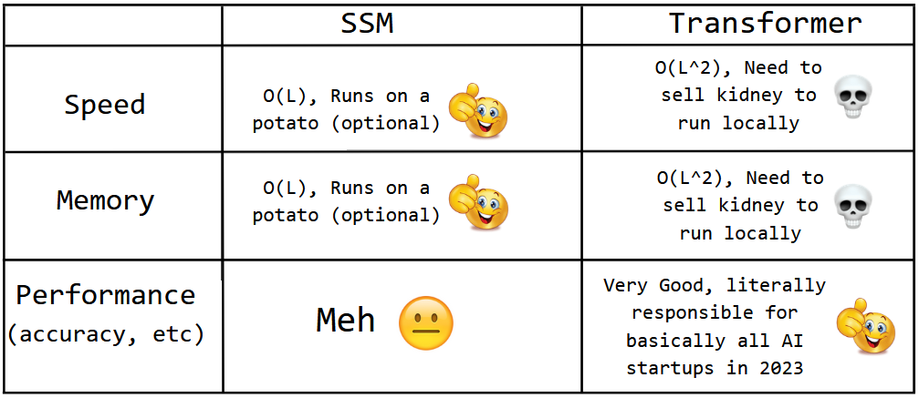
The main issue with multi-head attention sprouts from the fact that for input sequence length n, the time complexity and space complexity scales by O(n²). This limits the length of the context window of an LLM. Because, to increase it by 10x, we need to scale the hardware requirement (most notably GPU VRAM) by 100x.
Mamba, on the other hand, scales by O(n)!, i.e., Linearly.
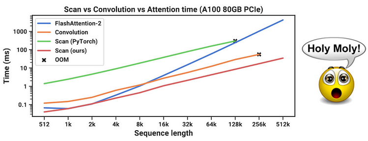
This linear scaling is what has taken wind for researchers to speculate that Mamba might be the future of sequence modeling.
The backbone of Mamba: State Space Models
The core of the Mamba model comes from the concept of State Space Models. State Space Models, like Transformers and RNN, process sequences of information, like text, audio signals, video frames, DNA sequences, etc.
State Space Models come from an idea of describing a physical system as a set of input, outputs, and variables. These variables are: A, B, C, D. The process of SSM involves calculation of an internal state vector h(t), given an input x(t). Then, we do a weighted sum of h(t) and x(t) where the weights are A, B, C, & D. In the simplest form (continuous time-invariant), the process formulation looks like:
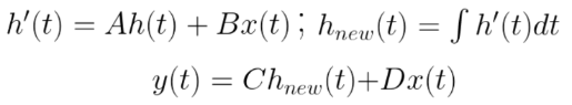
h(t) is often called the ‘hidden’ or the ‘latent’ state, I will be sticking to calling it the ‘hidden’ state for better clarity. It is important to note that A, B, C, and D are learnt parameters in SSM.
What are the variables?
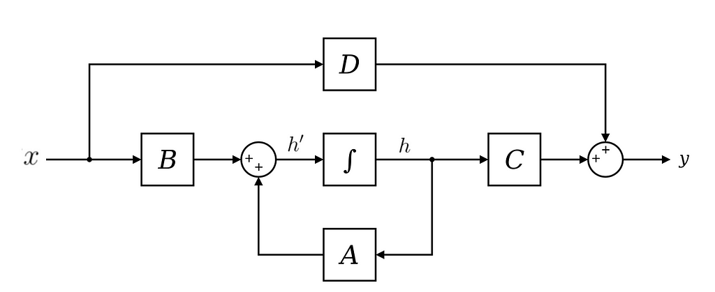
The variables, A, B, C & D, are learnt parameters, and they can be described as:
- A: How much should the previous hidden state (h) be considered to calculate the new hidden state
- B: How much should the input (x) be consider to calculate the new hidden state.
- C: How much should the new hidden state be considered in calculating the output (y).
- D: How much should the input (x) be consider in calculating the output (y).
D comes in the end of the computations and does not affect how the hidden state is calculated. Hence, it is usually considered outside of ssm, and can be thought of as a skip connection.
Going from continuous spaces to discrete spaces
The above formulation applies to a system where the input and output belong to a continuous space. But in cases, like language modeling, where the input and output belong to discrete spaces (token values in a vocabulary). Also, finding h(t) is analytically challenging. This can be achieved by performing a Zero-order hold.
In a zero-order hold, every time an input is received, the model holds its value till the next input is received. This leads to a continuous input space.
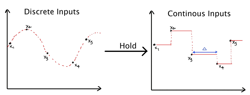
This length of ‘hold’ is determined by a new parameter called, step size ∆. It can be thought of as the resolution of the input. Ideally, ∆ should be infinitesimal.
Mathematically, Zero-order hold can be described as:
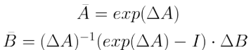
Finally, we can create a discrete SSM, as:
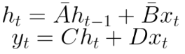
Since, D is used with a skip connection outside of SSM, the output can be reduced to:
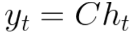

SSM and recurrence
In SSMs, the hidden state is carried over to when the next input is received. This is similar to how Recurrent Neural Networks function.
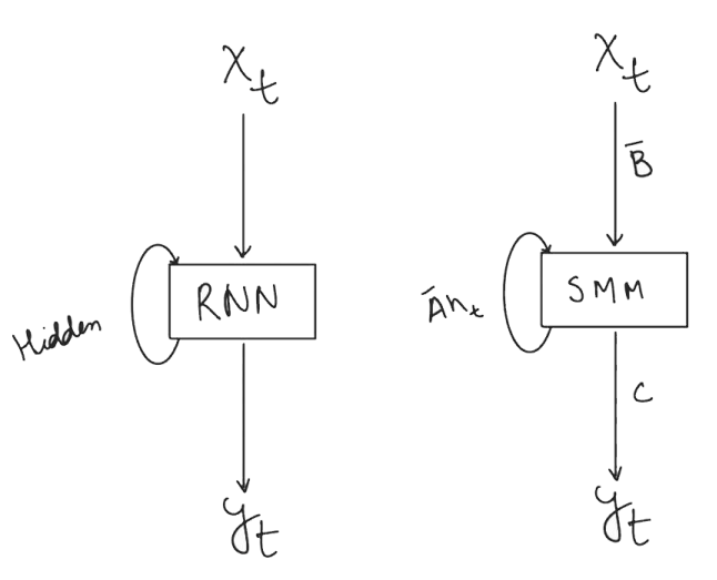
This recurrent format of SSM can be unwrapped, just like RNNs. But unlike RNNs, which are iterative and slow, SSM can process the input sequence in parallel (just like transformers) and this makes the training processes faster.
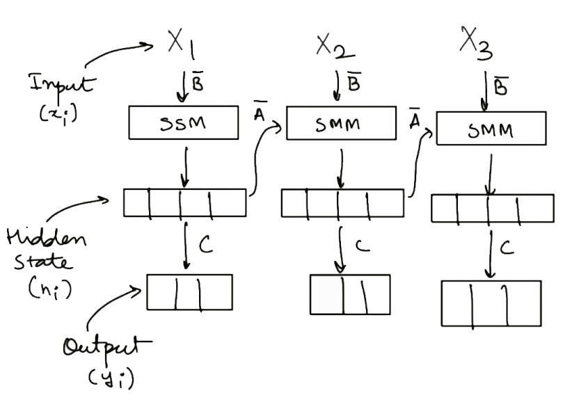
Note that ‘D’ is used in a skip connection, which is outside of SSM.
The key insight in how SSM make training fast is to use the variables A, B, C in a pre-computed convolutional kernel. Maarten Grootendorst wrote a really good explanation on how this canonical ‘convolutional’ kernel is constructed. But here’s a simple mathematical explanation.
Consider the output y. For a sequence length of k, the output for y(k) will be represented (assuming h0 = zero):
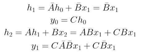
Similarly, y3 can be represented as:
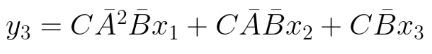
Extrapolating the pattern, yk can be represented as:

This formulation can be further reduced to:

The funny looking multiplication symbol represents a convolution operation, where the convolution kernel is K. Notice that K is not dependent on x, hence K can be pre-computed into a convolutional kernel, which makes the process faster.
Mamba and ‘Selective’ SSM
As good as the computational capacity of SSM sounds, it turns out to be pretty meh in metrics like accuracy compared to Transformers.
The core issue lies with the variables, ∆, A, B, & C. Turns out that since we apply the same matrices to every input, they cannot really process the context of the sequence.
SSMs are inflexible in the way they process data[4]
So what’s so special about Mamba? In mamba, we use a process called ‘selective’ SSM, where the variables, ∆, B, & C, are computed based on the input. 🤔. We do this by passing the current input through Linear layers, and take the output to be the ∆, B, & C.
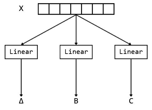
But then this makes ∆, B, & C input dependent, hence meaning that they cannot be pre-computed 😢, fast convolution isn’t going to work here. But, the authors discuss a method, which is based on parallel associative scan.
Parallel Associative Scan
Parallel associative scan is a powerful technique used in parallel computing to perform a prefix sum operation, which is a cumulative operation on a sequence of numbers. This operation is “associative”, meaning the way numbers are grouped in the operation doesn’t change the result.
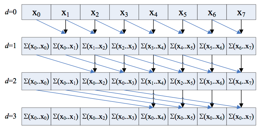
In the context of the Mamba model, by defining an associative operator, elements and associative operators for a parallel associative scan operation are obtained. This allows for solving problems on the whole time interval in parallel, resulting in logarithmic time complexity in the number of sub-intervals.
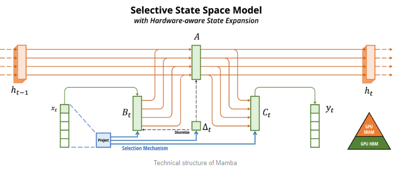
Hardware aware algorithm
Along with associative scan, the authors also propose a hardware aware algorithm, where they use the quirks within Nvidia GPUs related to the speed of HBM and SRAM. They argue that the computation of SSM states can be sped up by:
- keeping the hidden state and A in the faster but less capacity SRAM,
- while computing ∆, B, & C, in the slower but larger capacity HBM.
- They then transfer ∆, B, & C to the SRAM, compute the new hidden state within SRAM.
- And then write ∆, B & C back to HBM.
In the implementation section, I will not be discussing on how to work with the hardware aware algorithm, rather I will be only using parallel associative scan.
Final Mamba architecture
With all of this in mind, let’s explore and implement the Mamba architecture using Keras and TensorFlow.
The Mamba architecture, after reading the paper and analysis of the code, can be broken into a few key components which are connected as:
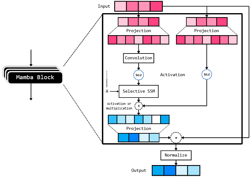
The Mamba architecture consists of multiple stacked layers of ‘Mamba blocks’. Which, judging from the above illustration, consists of quite a few components. Another important thing to note is that the authors add the output from Selective SSM to the original input and then apply a normalization layer to it. This normalization can be either a Layer normalization or an RMS normalization.
TensorFlow and Keras implementation
Lets start with coding part of Mamba. We will using the following dependencies:
tensorflow[and-cuda]==2.15.0.post1 # if you want to use GPU or
tensorflow==2.15.0.post1 # if you want to only use CPU
transformers==4.36.2 # for using the bert tokenizer
einops==0.7.0 # useful to make matrix manipulation faster
datasets==2.16.1 # to load datasets
# all other modules (like numpy) will be auto installed
Imports:
import tensorflow_datasets as tfds
import tensorflow as tf

from tensorflow import keras
from tensorflow.keras import layers, Model

from dataclasses import dataclass
from einops import rearrange, repeat
from typing import Union

from transformers import AutoTokenizer

import datasets
import math
import numpy as np
To make the modeling argument processing easier, let’s create a simple ModelArgs dataclass as a config class. This allows us to just pass the dataclass variable in the arguments when we are initializing the model.
@dataclass
class ModelArgs:
    model_input_dims: int = 64
    model_states: int = 64
    projection_expand_factor: int = 2
    conv_kernel_size: int = 4
    delta_t_min: float = 0.001
    delta_t_max: float = 0.1
    delta_t_scale: float = 0.1
    delta_t_init_floor: float = 1e-4
    conv_use_bias: bool = True
    dense_use_bias: bool = False
    layer_id: int = -1
    seq_length: int = 128
    num_layers: int = 5
    dropout_rate: float = 0.2
    use_lm_head: float = False
    num_classes: int = None
    vocab_size: int = None
    final_activation = None
    loss:Union[str, keras.losses.Loss] = None
    optimizer: Union[str, keras.optimizers.Optimizer] = keras.optimizers.AdamW()
    metrics = ['accuracy']

    def __post_init__(self):
        self.model_internal_dim: int = int(self.projection_expand_factor * self.model_input_dims)

        self.delta_t_rank = math.ceil(self.model_input_dims/16)
        if self.layer_id == -1:
            self.layer_id = np.round(np.random.randint(0, 1000), 4)

        if self.vocab_size == None:
            raise ValueError("vocab size cannot be none")

        if self.use_lm_head:
            self.num_classes=self.vocab_size
        else:
            if self.num_classes == None:
                raise ValueError(f'num classes cannot be {self.num_classes}')

            if self.num_classes == 1:
                self.final_activation = 'sigmoid'
            else:
                self.final_activation = 'softmax'

        if self.loss == None:
            raise ValueError(f"loss cannot be {self.loss}")
Load the bert-base-uncased tokenizer:
tokenizer = AutoTokenizer.from_pretrained("bert-base-uncased")
vocab_size = tokenizer.vocab_size
Before we implement our Mamba and SSM classes, we need to implement the parallel associative scan, the code looks like this:
def selective_scan(u, delta, A, B, C, D):
    # first step of A_bar = exp(ΔA), i.e., ΔA
    dA = tf.einsum('bld,dn->bldn', delta, A)
    dB_u = tf.einsum('bld,bld,bln->bldn', delta, u, B)

    dA_cumsum = tf.pad(
        dA[:, 1:], [[0, 0], [1, 1], [0, 0], [0, 0]])[:, 1:, :, :]

    dA_cumsum = tf.reverse(dA_cumsum, axis=[1])  # Flip along axis 1

    # Cumulative sum along all the input tokens, parallel prefix sum,
    # calculates dA for all the input tokens parallely
    dA_cumsum = tf.math.cumsum(dA_cumsum, axis=1)

    # second step of A_bar = exp(ΔA), i.e., exp(ΔA)
    dA_cumsum = tf.exp(dA_cumsum)
    dA_cumsum = tf.reverse(dA_cumsum, axis=[1])  # Flip back along axis 1

    x = dB_u * dA_cumsum
    # 1e-12 to avoid division by 0
    x = tf.math.cumsum(x, axis=1)/(dA_cumsum + 1e-12)

    y = tf.einsum('bldn,bln->bld', x, C)

    return y + u * D
With this, we can implement the MambaBlock:
class MambaBlock(layers.Layer):
    def __init__(self, modelargs: ModelArgs, *args, **kwargs):
        super().__init__(*args, **kwargs)
        self.args = modelargs
        args = modelargs
        self.layer_id = modelargs.layer_id

        self.in_projection = layers.Dense(
            args.model_internal_dim * 2,
            input_shape=(args.model_input_dims,), use_bias=False)

        self.conv1d = layers.Conv1D(
            filters=args.model_internal_dim,
            use_bias=args.conv_use_bias,
            kernel_size=args.conv_kernel_size,
            groups=args.model_internal_dim,
            data_format='channels_first',
            padding='causal'
        )

        # this layer takes in current token 'x'
        # and outputs the input-specific Δ, B, C (according to S6)
        self.x_projection = layers.Dense(args.delta_t_rank + args.model_states * 2, use_bias=False)

        # this layer projects Δ from delta_t_rank to the mamba internal
        # dimension
        self.delta_t_projection = layers.Dense(args.model_internal_dim,
                                               input_shape=(args.delta_t_rank,), use_bias=True)

        self.A = repeat(
                tf.range(1, args.model_states+1, dtype=tf.float32),
                'n -> d n', d=args.model_internal_dim)

        self.A_log = tf.Variable(
                tf.math.log(self.A),
                trainable=True, dtype=tf.float32,
                name=f"SSM_A_log_{args.layer_id}")

        self.D = tf.Variable(
                np.ones(args.model_internal_dim),
                trainable=True, dtype=tf.float32,
                name=f"SSM_D_{args.layer_id}")

        self.out_projection = layers.Dense(
                args.model_input_dims,
                input_shape=(args.model_internal_dim,),
                use_bias=args.dense_use_bias)

    def call(self, x):
        """Mamba block forward. This looks the same as Figure 3 in Section 3.4 in the Mamba pape.
        Official Implementation:
            class Mamba, https://github.com/state-spaces/mamba/blob/main/mamba_ssm/modules/mamba_simple.py#L119
            mamba_inner_ref(), https://github.com/state-spaces/mamba/blob/main/mamba_ssm/ops/selective_scan_interface.py#L311
        """

        (batch_size, seq_len, dimension) = x.shape

        x_and_res = self.in_projection(x) # shape = (batch, seq_len, 2 * model_internal_dimension)
        (x, res) = tf.split(x_and_res,
                            [self.args.model_internal_dim,
                             self.args.model_internal_dim], axis=-1)

        x = rearrange(x, 'b l d_in -> b d_in l')
        x = self.conv1d(x)[:, :, :seq_len]
        x = rearrange(x, 'b d_in l -> b l d_in')

        x = tf.nn.swish(x)
        y = self.ssm(x)
        y = y * tf.nn.swish(res)
        return self.out_projection(y)

    def ssm(self, x):
        """Runs the SSM. See:
            - Algorithm 2 in Section 3.2 in the Mamba paper
            - run_SSM(A, B, C, u) in The Annotated S4
            Official Implementation:
            mamba_inner_ref(), https://github.com/state-spaces/mamba/blob/main/mamba_ssm/ops/selective_scan_interface.py#L311
        """
        (d_in, n) = self.A_log.shape

        # Compute ∆ A B C D, the state space parameters.
        #     A, D are input independent (see Mamba paper [1] Section 3.5.2 "Interpretation of A" for why A isn't selective)
        #     ∆, B, C are input-dependent (this is a key difference between Mamba and the linear time invariant S4,
        #                                  and is why Mamba is called **selective** state spaces)

        A = -tf.exp(tf.cast(self.A_log, tf.float32)) # shape -> (d_in, n)
        D = tf.cast(self.D, tf.float32)

        x_dbl = self.x_projection(x) # shape -> (batch, seq_len, delta_t_rank + 2*n)

        (delta, B, C) = tf.split(
                x_dbl,
                num_or_size_splits=[self.args.delta_t_rank, n, n],
                axis=-1) # delta.shape -> (batch, seq_len) & B, C shape -> (batch, seq_len, n)

        delta = tf.nn.softplus(self.delta_t_projection(delta)) # shape -> (batch, seq_len, model_input_dim)

        return selective_scan(x, delta, A, B, C, D)
Finally, a residual block to implement the external skip connection.
class ResidualBlock(layers.Layer):
    def __init__(self, modelargs: ModelArgs, *args, **kwargs):
        super().__init__(*args, **kwargs)
        self.args = modelargs
        self.mixer = MambaBlock(modelargs)
        self.norm = layers.LayerNormalization(epsilon=1e-5)

    def call(self, x):
        """
        Official Implementation:
            Block.forward(), https://github.com/state-spaces/mamba/blob/main/mamba_ssm/modules/mamba_simple.py#L297

            Note: the official repo chains residual blocks that look like
                [Add -> Norm -> Mamba] -> [Add -> Norm -> Mamba] -> [Add -> Norm -> Mamba] -> ...
            where the first Add is a no-op. This is purely for performance reasons as this
            allows them to fuse the Add->Norm.

            We instead implement our blocks as the more familiar, simpler, and numerically equivalent
                [Norm -> Mamba -> Add] -> [Norm -> Mamba -> Add] -> [Norm -> Mamba -> Add] -> ....

        """
        return self.mixer(self.norm(x)) + x
With this, we can initialize our model. In this example, I will be demonstrating how to use the Mamba block to create a simple classification model, but it can be easily modified to become a language model. Let’s load the IMDB reviews dataset for a simple sentiment classifier.
from datasets import load_dataset
from tqdm import tqdm

dataset = load_dataset("ajaykarthick/imdb-movie-reviews")
First we create a function that will take the model args and return a model.
def init_model(args: ModelArgs):
    input_layer = layers.Input(shape=(args.seq_length,), name='input_ids')
    x = layers.Embedding(
                args.vocab_size,
                args.model_input_dims,
                input_length=args.seq_length)(input_layer)

    for i in range(args.num_layers):
        x = ResidualBlock(args, name=f"Residual_{i}")(x)
        x = layers.Dropout(args.dropout_rate)(x) # for regularization

    x = layers.LayerNormalization(epsilon=1e-5)(x) # normalization layer

    # use flatten only if we are not using the model as an LM
    if not args.use_lm_head:
        x = layers.Flatten()(x)
    x = layers.Dense(1024, activation=tf.nn.gelu)(x)
    output_layer = layers.Dense(
                args.num_classes,
                activation=args.final_activation)(x)

    model = Model(
                inputs=input_layer,
                outputs=output_layer, name='Mamba_ka_Mamba')
    model.compile(
        loss=args.loss,
        optimizer=args.optimizer,
        metrics=args.metrics
    )

    return model
Now we can initialize our model, and summarize it:
args = ModelArgs(
    model_input_dims=128,
    model_states=32,
    num_layers=12,
    dropout_rate=0.2,
    vocab_size=vocab_size,
    num_classes=1,
    loss='binary_crossentropy',
)
model = init_model(args)
model.summary()
Model: "Mamba_ka_Mamba"
_________________________________________________________________
 Layer (type)                Output Shape              Param #
=================================================================
 input_ids (InputLayer)      [(None, 128)]             0

 embedding_2 (Embedding)     (None, 128, 128)          3906816

 Residual_0 (ResidualBlock)  (None, 128, 128)          129024

 dropout_24 (Dropout)        (None, 128, 128)          0

 Residual_1 (ResidualBlock)  (None, 128, 128)          129024

 dropout_25 (Dropout)        (None, 128, 128)          0

 ... (I have shrinked this to make it more readable)

 dropout_35 (Dropout)        (None, 128, 128)          0

 layer_normalization_38 (La  (None, 128, 128)          256
 yerNormalization)

 flatten_2 (Flatten)         (None, 16384)             0

 dense_148 (Dense)           (None, 1024)              16778240

 dense_149 (Dense)           (None, 1)                 1025

=================================================================
Total params: 22234625 (84.82 MB)
Trainable params: 22234625 (84.82 MB)
Non-trainable params: 0 (0.00 Byte)
_________________________________________________________________
For easier processing, lets pre-tokenize our data into a numpy arrays, then convert them into tf.data.Dataset objects:
train_labels, test_labels = [], []
train_ids = np.zeros((len(dataset['train']), args.seq_length))
test_ids = np.zeros((len(dataset['test']), args.seq_length))

for i, item in enumerate(tqdm(dataset['train'])):
    text = item['review']
    train_ids[i, :] = tokenizer.encode_plus(
            text,
            max_length=args.seq_length,
            padding='max_length',
            return_tensors='np')['input_ids'][0][:args.seq_length]

    train_labels.append(item['label'])

for i, item in enumerate(tqdm(dataset['test'])):
    text = item['review']
    test_ids[i, :] = tokenizer.encode_plus(
            text,
            max_length=args.seq_length,
            padding='max_length',
            return_tensors='np')['input_ids'][0][:args.seq_length]

    test_labels.append(item['label'])

del dataset # delete the original dataset to save some memory

BATCH_SIZE = 32
train_dataset = tf.data.Dataset.from_tensor_slices((train_ids, train_labels)).batch(BATCH_SIZE).shuffle(1000)
test_dataset = tf.data.Dataset.from_tensor_slices((test_ids, test_labels)).batch(BATCH_SIZE).shuffle(1000)
Now the model can be trained:
history = model.fit(train_dataset, validation_data=test_dataset, epochs=10)
You can play around with the inference algorithm:
def infer(text: str, model: Model, tokenizer):
    tokens = tokenizer.encode(
            "Hello what is up",
            max_length=args.seq_length,
            padding='max_length', return_tensors='np')
    output = model(tokens)[0, 0]
    return output
This model can be converted into a language model and algorithms like beam search, top-k sampling, greedy sampling, etc. can be used to generate language.
This code can be found on my Github.
A lot of the code is inspired from the mamba’s official implementation[2] and another pytorch implementation called ‘mamba-tiny’[3]
Thank you for reading.
- Unless otherwise noted, all images are made by me.
References:
- Mamba paper.
- Mamba original repository
- A simpler Torch implementation of Mamba: mamba-tiny
- A simple explanation by Letitia on YouTube.
- Maarten Grootendorst’s article on SSMs and Mamba
- SSMs on wikipedia
- Nvidia’s tutorial on Parallel associative scan
Want to connect? Please write to me at [email protected]
Mamba: SSM, Theory, and Implementation in Keras and TensorFlow was originally published in Towards Data Science on Medium, where people are continuing the conversation by highlighting and responding to this story.
Understanding how SSMs and Mamba work, along with how to get started with implementing it in Keras and TensorFlow.

Submitted on 1st December, 2023 on arXiv, the paper titled “Mamba: Linear-Time Sequence Modeling with Selective State Spaces” proposed an interesting approach to sequence modeling. The authors — Albert Gu, Tri Dao — introduced, ‘Mamba’ that utilized ‘selective’ state space models (SSM) to achieve results that compete with the performance of the, now ubiquitous, Transformer model.
What’s so unique about Mamba?
Transformers have seen recent popularity with the rise of Large Language Models (LLMs) like LLaMa-2, GPT-4, Claude, Gemini, etc., but it suffers from the problem of context window. The issue with transformers lies in it’s core, the multi head-attention mechanism.
The main issue with multi-head attention sprouts from the fact that for input sequence length n, the time complexity and space complexity scales by O(n²). This limits the length of the context window of an LLM. Because, to increase it by 10x, we need to scale the hardware requirement (most notably GPU VRAM) by 100x.
Mamba, on the other hand, scales by O(n)!, i.e., Linearly.
This linear scaling is what has taken wind for researchers to speculate that Mamba might be the future of sequence modeling.
The backbone of Mamba: State Space Models
The core of the Mamba model comes from the concept of State Space Models. State Space Models, like Transformers and RNN, process sequences of information, like text, audio signals, video frames, DNA sequences, etc.
State Space Models come from an idea of describing a physical system as a set of input, outputs, and variables. These variables are: A, B, C, D. The process of SSM involves calculation of an internal state vector h(t), given an input x(t). Then, we do a weighted sum of h(t) and x(t) where the weights are A, B, C, & D. In the simplest form (continuous time-invariant), the process formulation looks like:
h(t) is often called the ‘hidden’ or the ‘latent’ state, I will be sticking to calling it the ‘hidden’ state for better clarity. It is important to note that A, B, C, and D are learnt parameters in SSM.
What are the variables?
The variables, A, B, C & D, are learnt parameters, and they can be described as:
- A: How much should the previous hidden state (h) be considered to calculate the new hidden state
- B: How much should the input (x) be consider to calculate the new hidden state.
- C: How much should the new hidden state be considered in calculating the output (y).
- D: How much should the input (x) be consider in calculating the output (y).
D comes in the end of the computations and does not affect how the hidden state is calculated. Hence, it is usually considered outside of ssm, and can be thought of as a skip connection.
Going from continuous spaces to discrete spaces
The above formulation applies to a system where the input and output belong to a continuous space. But in cases, like language modeling, where the input and output belong to discrete spaces (token values in a vocabulary). Also, finding h(t) is analytically challenging. This can be achieved by performing a Zero-order hold.
In a zero-order hold, every time an input is received, the model holds its value till the next input is received. This leads to a continuous input space.
This length of ‘hold’ is determined by a new parameter called, step size ∆. It can be thought of as the resolution of the input. Ideally, ∆ should be infinitesimal.
Mathematically, Zero-order hold can be described as:
Finally, we can create a discrete SSM, as:
Since, D is used with a skip connection outside of SSM, the output can be reduced to:
SSM and recurrence
In SSMs, the hidden state is carried over to when the next input is received. This is similar to how Recurrent Neural Networks function.
This recurrent format of SSM can be unwrapped, just like RNNs. But unlike RNNs, which are iterative and slow, SSM can process the input sequence in parallel (just like transformers) and this makes the training processes faster.
Note that ‘D’ is used in a skip connection, which is outside of SSM.
The key insight in how SSM make training fast is to use the variables A, B, C in a pre-computed convolutional kernel. Maarten Grootendorst wrote a really good explanation on how this canonical ‘convolutional’ kernel is constructed. But here’s a simple mathematical explanation.
Consider the output y. For a sequence length of k, the output for y(k) will be represented (assuming h0 = zero):
Similarly, y3 can be represented as:
Extrapolating the pattern, yk can be represented as:
This formulation can be further reduced to:
The funny looking multiplication symbol represents a convolution operation, where the convolution kernel is K. Notice that K is not dependent on x, hence K can be pre-computed into a convolutional kernel, which makes the process faster.
Mamba and ‘Selective’ SSM
As good as the computational capacity of SSM sounds, it turns out to be pretty meh in metrics like accuracy compared to Transformers.
The core issue lies with the variables, ∆, A, B, & C. Turns out that since we apply the same matrices to every input, they cannot really process the context of the sequence.
SSMs are inflexible in the way they process data[4]
So what’s so special about Mamba? In mamba, we use a process called ‘selective’ SSM, where the variables, ∆, B, & C, are computed based on the input. 🤔. We do this by passing the current input through Linear layers, and take the output to be the ∆, B, & C.
But then this makes ∆, B, & C input dependent, hence meaning that they cannot be pre-computed 😢, fast convolution isn’t going to work here. But, the authors discuss a method, which is based on parallel associative scan.
Parallel Associative Scan
Parallel associative scan is a powerful technique used in parallel computing to perform a prefix sum operation, which is a cumulative operation on a sequence of numbers. This operation is “associative”, meaning the way numbers are grouped in the operation doesn’t change the result.
In the context of the Mamba model, by defining an associative operator, elements and associative operators for a parallel associative scan operation are obtained. This allows for solving problems on the whole time interval in parallel, resulting in logarithmic time complexity in the number of sub-intervals.
Hardware aware algorithm
Along with associative scan, the authors also propose a hardware aware algorithm, where they use the quirks within Nvidia GPUs related to the speed of HBM and SRAM. They argue that the computation of SSM states can be sped up by:
- keeping the hidden state and A in the faster but less capacity SRAM,
- while computing ∆, B, & C, in the slower but larger capacity HBM.
- They then transfer ∆, B, & C to the SRAM, compute the new hidden state within SRAM.
- And then write ∆, B & C back to HBM.
In the implementation section, I will not be discussing on how to work with the hardware aware algorithm, rather I will be only using parallel associative scan.
Final Mamba architecture
With all of this in mind, let’s explore and implement the Mamba architecture using Keras and TensorFlow.
The Mamba architecture, after reading the paper and analysis of the code, can be broken into a few key components which are connected as:
The Mamba architecture consists of multiple stacked layers of ‘Mamba blocks’. Which, judging from the above illustration, consists of quite a few components. Another important thing to note is that the authors add the output from Selective SSM to the original input and then apply a normalization layer to it. This normalization can be either a Layer normalization or an RMS normalization.
TensorFlow and Keras implementation
Lets start with coding part of Mamba. We will using the following dependencies:
tensorflow[and-cuda]==2.15.0.post1 # if you want to use GPU or
tensorflow==2.15.0.post1 # if you want to only use CPU
transformers==4.36.2 # for using the bert tokenizer
einops==0.7.0 # useful to make matrix manipulation faster
datasets==2.16.1 # to load datasets
# all other modules (like numpy) will be auto installed
Imports:
import tensorflow_datasets as tfds
import tensorflow as tf

from tensorflow import keras
from tensorflow.keras import layers, Model

from dataclasses import dataclass
from einops import rearrange, repeat
from typing import Union

from transformers import AutoTokenizer

import datasets
import math
import numpy as np
To make the modeling argument processing easier, let’s create a simple ModelArgs dataclass as a config class. This allows us to just pass the dataclass variable in the arguments when we are initializing the model.
@dataclass
class ModelArgs:
    model_input_dims: int = 64
    model_states: int = 64
    projection_expand_factor: int = 2
    conv_kernel_size: int = 4
    delta_t_min: float = 0.001
    delta_t_max: float = 0.1
    delta_t_scale: float = 0.1
    delta_t_init_floor: float = 1e-4
    conv_use_bias: bool = True
    dense_use_bias: bool = False
    layer_id: int = -1
    seq_length: int = 128
    num_layers: int = 5
    dropout_rate: float = 0.2
    use_lm_head: float = False
    num_classes: int = None
    vocab_size: int = None
    final_activation = None
    loss:Union[str, keras.losses.Loss] = None
    optimizer: Union[str, keras.optimizers.Optimizer] = keras.optimizers.AdamW()
    metrics = ['accuracy']

    def __post_init__(self):
        self.model_internal_dim: int = int(self.projection_expand_factor * self.model_input_dims)

        self.delta_t_rank = math.ceil(self.model_input_dims/16)
        if self.layer_id == -1:
            self.layer_id = np.round(np.random.randint(0, 1000), 4)

        if self.vocab_size == None:
            raise ValueError("vocab size cannot be none")

        if self.use_lm_head:
            self.num_classes=self.vocab_size
        else:
            if self.num_classes == None:
                raise ValueError(f'num classes cannot be {self.num_classes}')

            if self.num_classes == 1:
                self.final_activation = 'sigmoid'
            else:
                self.final_activation = 'softmax'

        if self.loss == None:
            raise ValueError(f"loss cannot be {self.loss}")
Load the bert-base-uncased tokenizer:
tokenizer = AutoTokenizer.from_pretrained("bert-base-uncased")
vocab_size = tokenizer.vocab_size
Before we implement our Mamba and SSM classes, we need to implement the parallel associative scan, the code looks like this:
def selective_scan(u, delta, A, B, C, D):
    # first step of A_bar = exp(ΔA), i.e., ΔA
    dA = tf.einsum('bld,dn->bldn', delta, A)
    dB_u = tf.einsum('bld,bld,bln->bldn', delta, u, B)

    dA_cumsum = tf.pad(
        dA[:, 1:], [[0, 0], [1, 1], [0, 0], [0, 0]])[:, 1:, :, :]

    dA_cumsum = tf.reverse(dA_cumsum, axis=[1])  # Flip along axis 1

    # Cumulative sum along all the input tokens, parallel prefix sum,
    # calculates dA for all the input tokens parallely
    dA_cumsum = tf.math.cumsum(dA_cumsum, axis=1)

    # second step of A_bar = exp(ΔA), i.e., exp(ΔA)
    dA_cumsum = tf.exp(dA_cumsum)
    dA_cumsum = tf.reverse(dA_cumsum, axis=[1])  # Flip back along axis 1

    x = dB_u * dA_cumsum
    # 1e-12 to avoid division by 0
    x = tf.math.cumsum(x, axis=1)/(dA_cumsum + 1e-12)

    y = tf.einsum('bldn,bln->bld', x, C)

    return y + u * D
With this, we can implement the MambaBlock:
class MambaBlock(layers.Layer):
    def __init__(self, modelargs: ModelArgs, *args, **kwargs):
        super().__init__(*args, **kwargs)
        self.args = modelargs
        args = modelargs
        self.layer_id = modelargs.layer_id

        self.in_projection = layers.Dense(
            args.model_internal_dim * 2,
            input_shape=(args.model_input_dims,), use_bias=False)

        self.conv1d = layers.Conv1D(
            filters=args.model_internal_dim,
            use_bias=args.conv_use_bias,
            kernel_size=args.conv_kernel_size,
            groups=args.model_internal_dim,
            data_format='channels_first',
            padding='causal'
        )

        # this layer takes in current token 'x'
        # and outputs the input-specific Δ, B, C (according to S6)
        self.x_projection = layers.Dense(args.delta_t_rank + args.model_states * 2, use_bias=False)

        # this layer projects Δ from delta_t_rank to the mamba internal
        # dimension
        self.delta_t_projection = layers.Dense(args.model_internal_dim,
                                               input_shape=(args.delta_t_rank,), use_bias=True)

        self.A = repeat(
                tf.range(1, args.model_states+1, dtype=tf.float32),
                'n -> d n', d=args.model_internal_dim)

        self.A_log = tf.Variable(
                tf.math.log(self.A),
                trainable=True, dtype=tf.float32,
                name=f"SSM_A_log_{args.layer_id}")

        self.D = tf.Variable(
                np.ones(args.model_internal_dim),
                trainable=True, dtype=tf.float32,
                name=f"SSM_D_{args.layer_id}")

        self.out_projection = layers.Dense(
                args.model_input_dims,
                input_shape=(args.model_internal_dim,),
                use_bias=args.dense_use_bias)

    def call(self, x):
        """Mamba block forward. This looks the same as Figure 3 in Section 3.4 in the Mamba pape.
        Official Implementation:
            class Mamba, https://github.com/state-spaces/mamba/blob/main/mamba_ssm/modules/mamba_simple.py#L119
            mamba_inner_ref(), https://github.com/state-spaces/mamba/blob/main/mamba_ssm/ops/selective_scan_interface.py#L311
        """

        (batch_size, seq_len, dimension) = x.shape

        x_and_res = self.in_projection(x) # shape = (batch, seq_len, 2 * model_internal_dimension)
        (x, res) = tf.split(x_and_res,
                            [self.args.model_internal_dim,
                             self.args.model_internal_dim], axis=-1)

        x = rearrange(x, 'b l d_in -> b d_in l')
        x = self.conv1d(x)[:, :, :seq_len]
        x = rearrange(x, 'b d_in l -> b l d_in')

        x = tf.nn.swish(x)
        y = self.ssm(x)
        y = y * tf.nn.swish(res)
        return self.out_projection(y)

    def ssm(self, x):
        """Runs the SSM. See:
            - Algorithm 2 in Section 3.2 in the Mamba paper
            - run_SSM(A, B, C, u) in The Annotated S4
            Official Implementation:
            mamba_inner_ref(), https://github.com/state-spaces/mamba/blob/main/mamba_ssm/ops/selective_scan_interface.py#L311
        """
        (d_in, n) = self.A_log.shape

        # Compute ∆ A B C D, the state space parameters.
        #     A, D are input independent (see Mamba paper [1] Section 3.5.2 "Interpretation of A" for why A isn't selective)
        #     ∆, B, C are input-dependent (this is a key difference between Mamba and the linear time invariant S4,
        #                                  and is why Mamba is called **selective** state spaces)

        A = -tf.exp(tf.cast(self.A_log, tf.float32)) # shape -> (d_in, n)
        D = tf.cast(self.D, tf.float32)

        x_dbl = self.x_projection(x) # shape -> (batch, seq_len, delta_t_rank + 2*n)

        (delta, B, C) = tf.split(
                x_dbl,
                num_or_size_splits=[self.args.delta_t_rank, n, n],
                axis=-1) # delta.shape -> (batch, seq_len) & B, C shape -> (batch, seq_len, n)

        delta = tf.nn.softplus(self.delta_t_projection(delta)) # shape -> (batch, seq_len, model_input_dim)

        return selective_scan(x, delta, A, B, C, D)
Finally, a residual block to implement the external skip connection.
class ResidualBlock(layers.Layer):
    def __init__(self, modelargs: ModelArgs, *args, **kwargs):
        super().__init__(*args, **kwargs)
        self.args = modelargs
        self.mixer = MambaBlock(modelargs)
        self.norm = layers.LayerNormalization(epsilon=1e-5)

    def call(self, x):
        """
        Official Implementation:
            Block.forward(), https://github.com/state-spaces/mamba/blob/main/mamba_ssm/modules/mamba_simple.py#L297

            Note: the official repo chains residual blocks that look like
                [Add -> Norm -> Mamba] -> [Add -> Norm -> Mamba] -> [Add -> Norm -> Mamba] -> ...
            where the first Add is a no-op. This is purely for performance reasons as this
            allows them to fuse the Add->Norm.

            We instead implement our blocks as the more familiar, simpler, and numerically equivalent
                [Norm -> Mamba -> Add] -> [Norm -> Mamba -> Add] -> [Norm -> Mamba -> Add] -> ....

        """
        return self.mixer(self.norm(x)) + x
With this, we can initialize our model. In this example, I will be demonstrating how to use the Mamba block to create a simple classification model, but it can be easily modified to become a language model. Let’s load the IMDB reviews dataset for a simple sentiment classifier.
from datasets import load_dataset
from tqdm import tqdm

dataset = load_dataset("ajaykarthick/imdb-movie-reviews")
First we create a function that will take the model args and return a model.
def init_model(args: ModelArgs):
    input_layer = layers.Input(shape=(args.seq_length,), name='input_ids')
    x = layers.Embedding(
                args.vocab_size,
                args.model_input_dims,
                input_length=args.seq_length)(input_layer)

    for i in range(args.num_layers):
        x = ResidualBlock(args, name=f"Residual_{i}")(x)
        x = layers.Dropout(args.dropout_rate)(x) # for regularization

    x = layers.LayerNormalization(epsilon=1e-5)(x) # normalization layer

    # use flatten only if we are not using the model as an LM
    if not args.use_lm_head:
        x = layers.Flatten()(x)
    x = layers.Dense(1024, activation=tf.nn.gelu)(x)
    output_layer = layers.Dense(
                args.num_classes,
                activation=args.final_activation)(x)

    model = Model(
                inputs=input_layer,
                outputs=output_layer, name='Mamba_ka_Mamba')
    model.compile(
        loss=args.loss,
        optimizer=args.optimizer,
        metrics=args.metrics
    )

    return model
Now we can initialize our model, and summarize it:
args = ModelArgs(
    model_input_dims=128,
    model_states=32,
    num_layers=12,
    dropout_rate=0.2,
    vocab_size=vocab_size,
    num_classes=1,
    loss='binary_crossentropy',
)
model = init_model(args)
model.summary()
Model: "Mamba_ka_Mamba"
_________________________________________________________________
 Layer (type)                Output Shape              Param #
=================================================================
 input_ids (InputLayer)      [(None, 128)]             0

 embedding_2 (Embedding)     (None, 128, 128)          3906816

 Residual_0 (ResidualBlock)  (None, 128, 128)          129024

 dropout_24 (Dropout)        (None, 128, 128)          0

 Residual_1 (ResidualBlock)  (None, 128, 128)          129024

 dropout_25 (Dropout)        (None, 128, 128)          0

 ... (I have shrinked this to make it more readable)

 dropout_35 (Dropout)        (None, 128, 128)          0

 layer_normalization_38 (La  (None, 128, 128)          256
 yerNormalization)

 flatten_2 (Flatten)         (None, 16384)             0

 dense_148 (Dense)           (None, 1024)              16778240

 dense_149 (Dense)           (None, 1)                 1025

=================================================================
Total params: 22234625 (84.82 MB)
Trainable params: 22234625 (84.82 MB)
Non-trainable params: 0 (0.00 Byte)
_________________________________________________________________
For easier processing, lets pre-tokenize our data into a numpy arrays, then convert them into tf.data.Dataset objects:
train_labels, test_labels = [], []
train_ids = np.zeros((len(dataset['train']), args.seq_length))
test_ids = np.zeros((len(dataset['test']), args.seq_length))

for i, item in enumerate(tqdm(dataset['train'])):
    text = item['review']
    train_ids[i, :] = tokenizer.encode_plus(
            text,
            max_length=args.seq_length,
            padding='max_length',
            return_tensors='np')['input_ids'][0][:args.seq_length]

    train_labels.append(item['label'])

for i, item in enumerate(tqdm(dataset['test'])):
    text = item['review']
    test_ids[i, :] = tokenizer.encode_plus(
            text,
            max_length=args.seq_length,
            padding='max_length',
            return_tensors='np')['input_ids'][0][:args.seq_length]

    test_labels.append(item['label'])

del dataset # delete the original dataset to save some memory

BATCH_SIZE = 32
train_dataset = tf.data.Dataset.from_tensor_slices((train_ids, train_labels)).batch(BATCH_SIZE).shuffle(1000)
test_dataset = tf.data.Dataset.from_tensor_slices((test_ids, test_labels)).batch(BATCH_SIZE).shuffle(1000)
Now the model can be trained:
history = model.fit(train_dataset, validation_data=test_dataset, epochs=10)
You can play around with the inference algorithm:
def infer(text: str, model: Model, tokenizer):
    tokens = tokenizer.encode(
            "Hello what is up",
            max_length=args.seq_length,
            padding='max_length', return_tensors='np')
    output = model(tokens)[0, 0]
    return output
This model can be converted into a language model and algorithms like beam search, top-k sampling, greedy sampling, etc. can be used to generate language.
This code can be found on my Github.
A lot of the code is inspired from the mamba’s official implementation[2] and another pytorch implementation called ‘mamba-tiny’[3]
Thank you for reading.
- Unless otherwise noted, all images are made by me.
References:
- Mamba paper.
- Mamba original repository
- A simpler Torch implementation of Mamba: mamba-tiny
- A simple explanation by Letitia on YouTube.
- Maarten Grootendorst’s article on SSMs and Mamba
- SSMs on wikipedia
- Nvidia’s tutorial on Parallel associative scan
Want to connect? Please write to me at [email protected]
Mamba: SSM, Theory, and Implementation in Keras and TensorFlow was originally published in Towards Data Science on Medium, where people are continuing the conversation by highlighting and responding to this story.
Denial of responsibility! Techno Blender is an automatic aggregator of the all world’s media. In each content, the hyperlink to the primary source is specified. All trademarks belong to their rightful owners, all materials to their authors. If you are the owner of the content and do not want us to publish your materials, please contact us by email – [email protected]. The content will be deleted within 24 hours.