
Map-Matching for Speed Prediction
How fast will you drive?
When planning future vehicle routes, you trust the digital map providers for accurate speed predictions. You do this when picking your phone up to prepare for a car trip or, in a professional setting, when planning routes for your vehicle fleet. The forecasted speeds are an essential component of the trip’s cost, especially as they are one of the fundamental drivers of energy consumption in electric and combustion vehicles.
The digital mapping service providers collect information from live traffic and historical records to estimate how fast you can drive along a specific road at any given time. With this data and intelligent algorithms, they estimate how quickly an average vehicle will travel through the planned route. Some services will accept each vehicle’s features to tune the route path and the expected trip times.
But what about specific vehicles and drivers like yours? Do these predictions apply? Your cars and drivers might have particular requirements or habits that do not fit the standardized forecasts. Can we do better than the digital map service providers? We have a chance if you keep a good record of your historical telematics data.
Introduction
In this article, we will improve the quality of speed predictions from digital map providers by leveraging the historical speed profiles from a telematics database. This database contains records of past trips that we use to modulate the standard speed inferences from a digital map provider.
Central to this is map-matching, the process by which we “snap” the observed GPS locations to the underlying digital map. This correcting step allows us to bring the GPS measurements in line with the map’s road network representation, thus making all location sources comparable.
The Road Network
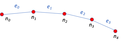
A road network is a mathematical concept that supports most digital mapping applications. Usually implemented as a directed multi-graph, each node represents a known geospatial location, usually some noteworthy landmark such as an intersection or a defining point on a road bend, and the connecting directed edges represent straight-line paths along the road. Figure 1 below illustrates the concept.
When we request a route from a digital map provider, we get a sequence of road network nodes and their connecting edges. The service also provides the estimated travel times and corresponding speeds between all pairs of nodes (in some cases, the speed estimates cover a range of nodes). We get the total trip duration by adding all the partial times together.
If we get better estimates for these times, we will also have better speed estimates and a better route prediction overall. The source for these better estimates is your historical telematics data. But knowing the historic speeds is just a part of the process. Before we can use these speeds, we must make sure that we can project them onto the digital map, and for this, we use map-matching.
Map-Matching
Map-matching projects sequences of GPS coordinates sampled from a moving object’s path to an existing road graph. The matching process uses a Hidden Markov Model to map the sampled locations to the most likely graph edge sequence. As a result, this process produces both the edge projections and the implicit node sequence. You can read a more detailed explanation in my previous article on map matching:
Map-Matching for Trajectory Prediction
After reading the above article, you will understand that the Valhalla map-matching algorithm projects the sampled GPS locations into road network edges, not to the nodes. The service may also return the matched poly-line defined in terms of the road network nodes. So, we can get both edge projections and the implicit node sequence.
On the other hand, when retrieving a route plan from the same provider, we also get a sequence of road network nodes. By matching these nodes to the previously map-matched ones, we can overlay the known telematics information to the newly generated route and thus improve the time and speed estimates with actual data.
Before using the map-matched locations to infer actual speeds, we must project them to the nodes and adjust the known travel times, as illustrated in Figure 2 below.
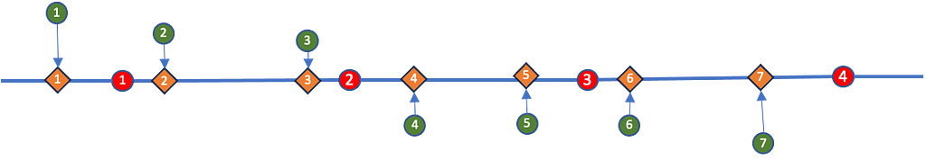
As a prerequisite, we must correctly sequence both sets of locations, the nodes, and the map matches. This process is depicted in Figure 2 above, where the map matches, represented by the orange diamonds, are sequenced along with the road network nodes, represented as red dots. The travel sequence is obviously from left to right.
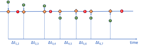
We assume the time differences between the GPS locations are the same as the map-matched ones. This assumption, illustrated by Figure 3 below, is essential because there is no way to infer what effect in time the map matching has. This assumption simplifies the calculation while keeping a good approximation.
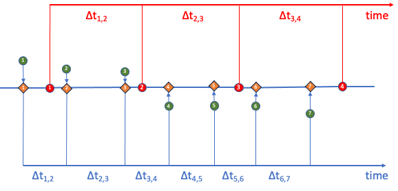
Now that we know the time differences between consecutive orange diamonds, our challenge is to use this information to infer the time differences between consecutive red dots (nodes). Figure 4 below shows the relationship between the two sequences of time differences.
We can safely assume that the average speeds between consecutive orange diamonds are constant. This assumption is essential for what comes next. But before we proceed, let’s define some terminology. We will use some simplifications due to Medium’s typesetting limitations.
We need to deal with two fundamental quantities: distances and timespans. Using Figure 4 above as a reference, we define the distance between the orange diamond one and red dot one as d(n1, m1). Here, the letter “m” stands for “map-matched,” and the letter “n” stands for node. Similarly, the corresponding timespan is t(n1, m1), and the average speed is v(n1, m1).
Let us focus on the first two nodes and see how we can derive the average speed (and the corresponding timespan) using the known timespans from orange diamonds one to four. The average speed of travel between the first two map-matched locations is thus:

Because the average speed is constant, we can now compute the first timespan.

The second timespan is just t(m2, m3). For the final period, we can repeat the process above. The total time is thus:

We must repeat this process, adapting it to the sequence of nodes and map matches to calculate the projected trip times between all nodes.
Now that we have seen how to project measured speeds onto a digital map let’s see where to get the data.
Telematics Database
This article uses a telematics database to infer unknown road segment average speeds. All the geospatial data in the database is already map-matched to the underlying digital map. This characteristic helps us match future service-provided routes to the known or projected road segment speeds using the abovementioned process.
Here, we will use a tried-and-true open-source telematics database I have been exploring lately and presented in a previously published article, the Extended Vehicle Energy Dataset (EVED), licensed under Apache 2.0.
Travel Time Estimation Using Quadkeys
Proposed Solution
We develop the solution in two steps: data preparation and prediction. In the data preparation step, we traverse all known trips in the telematics database and project the measured trip times to the corresponding road network edges. These computed edge traversal times are then stored in another database using maximum resolution H3 indices for faster searches during exploration. At the end of the process, we have collected traversal time distributions for the known edges, information that will allow us to estimate travel speeds in the prediction phase.
The prediction phase requires a source route expressed as a sequence of road network nodes, such as what we get from the Valhalla route planner. We query each pair of consecutive nodes' corresponding traversal time distribution (if any) from the speed database and use its mean (or median) to estimate the local average speed. By adding all edge estimates, we get the intended result, the expected total trip time.
Data Preparation
To prepare the data and generate the reference time distribution database, we must iterate through all the trips in the source data. Fortunately, the source database makes this easy by readily identifying all the trips (see the article above).
Let us look at the code that prepares the edge traversal times.
https://medium.com/media/d248980cdb01797aebfd16932fc03594/href
The code in Figure 5 above shows the main loop of the data preparation code. We use the previously created EVED database and save the output data to a new speed database. Each record is a time traversal sample for a single road network edge. For the same edge, a set of these samples makes up for a statistical time distribution, for which we calculate the average, median, and other statistics.
The call on line 5 retrieves a list of all the known trips in the source database as triplets containing the trajectory identifier (the table sequential identifier), the vehicle identifier, and the trip identifier. We need these last two items to retrieve the trip’s signals, as shown in line 10.
Lines 10 to 16 contain the code that retrieves the trip’s trajectory as a sequence of latitude, longitude, and timestamps. These locations do not necessarily correspond to road network nodes; they will mostly be projections into the edges (the orange diamonds in Figure 2).
Now, we can ask the Valhalla map-matching engine to take these points and return a poly-line with the corresponding road network node sequence, as shown in lines 18 to 25. These are the nodes that we store in the database, along with the projected traversal times, which we derive in the final lines of the code.
The traversal time projection from the map-matched locations to the node locations occurs in two steps. First, line 27 creates a “compound trajectory” object that merges the map-matched locations and the corresponding nodes in the trip sequence. The object stores each map-matched segment separately for later joining. Figure 6 below shows the object constructor (source file).
https://medium.com/media/20f2edca46fc9ab2acc9863324a535eb/href
The compound trajectory constructor starts by merging the sequence of map-matched points to the corresponding road network nodes. Referring to the symbols in Figure 2 above, the code combines the orange diamond sequence with the red dot sequence so they keep the trip order. In the first step, listed in Figure 7 below, we create a list of sequences of orange diamond pairs with any red dots in between.
https://medium.com/media/0b161ec19e1792caea41fc48dcadd0c4/href
Once merged, we convert the trajectory segments to node-based trajectories, removing the map-matched endpoints and recomputing the traversal times. Figure 8 below shows the function that computes the equivalent between-node traversal times.
https://medium.com/media/bfaae00ea29cf906f1132bb6b53c5396/href
Using the symbology of Figure 2, the code above uses the traversal times between two orange diamonds and calculates the times for all sub-segment traversals, namely between node-delimited ones. This way, we can later reconstruct all between-node traversal times through simple addition.
The final conversion step occurs on line 28 of Figure 5 when we convert the compound trajectory to a simple trajectory using the functions listed in Figure 9 below.
https://medium.com/media/1a614affe3d7a5f0155541949c36437a/href
The final step of the code in Figure 5 (lines 30–32) is to save the computed edge traversal times to the database for posterior use.
Data Quality
How good is the data that we just prepared? Does the EVED allow for good speed predictions? Unfortunately, this database was not designed for this purpose so that we will see some issues.
The first issue is the number of single-edge records in the final database, in this case, a little over two million. The total number of rows is over 5.6 million, so the unusable single-edge records represent a sizable proportion of the database. Almost half the rows are from edges with ten or fewer records.
The second issue is trips with very low frequencies. When querying an ad-hoc trip, we may fall into areas of very low density, where edge time records are scarce or nonexistent. In such conditions, the prediction code tries to compensate for the data loss using a simple heuristic: assume the same average speed as in the last edge. For larger road sections, and as we see below, we may even copy the data from the Valhalla route predictor.
The bottom line is that some of these predictions will be bad. A better use case for this algorithm would be to use a telematics database from fleets that frequently travel through the same routes. It would be even better to get more data for the same routes.
Prediction
To explore this time-prediction enhancement algorithm, we will use two different scripts: one interactive Streamlit application that allows you to freely use the map and an analytics script that tries to assess the quality of the predicted times by comparing them to known trip times in a LOOCV type of approach.
Interactive Map
You run the interactive application by executing the following command line at the project root:
streamlit run speed-predict.py
The interactive application allows you to specify endpoints of a route for Valhalla to predict. Figure 10 below shows what the user interface looks like.
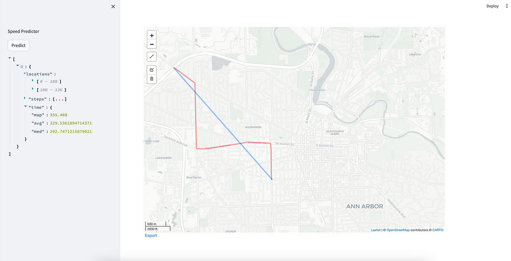
To operate the application, use the drawing button below the zoom control to select the source, destination, and optional waypoints. The application draws the sequence as a blue line, as depicted. Next, press the “Predict” button on the top left, under the title. The application calls the Valhalla route predictor and draws its result as a red line. To the left, you see some of the output, namely the time estimates of the map provider and the two below from the algorithm described here. The first estimate uses the average of the matching edge time distributions, and the second uses the median. For missing data, the algorithm uses the map estimate.
Note that the application draws a black rectangle around the area where data is available. Outside of that area, all predictions will be the same as the map’s.
Accuracy Estimator
To estimate the accuracy of this time predictor, we will test it against known trips taken from the database. We will match the edge projections to the corresponding map nodes for each sampled trip and then query their duration distributions, excluding the data from the trip we want to estimate. This is a process akin to the known Leave-One-Out Cross Validation process.
Use the following command line to invoke the accuracy estimator script:
python benchmark-trips.py
When finished, the script outputs the estimates to a CSV file that you can use for accuracy analysis, as illustrated in Figure 11 below.
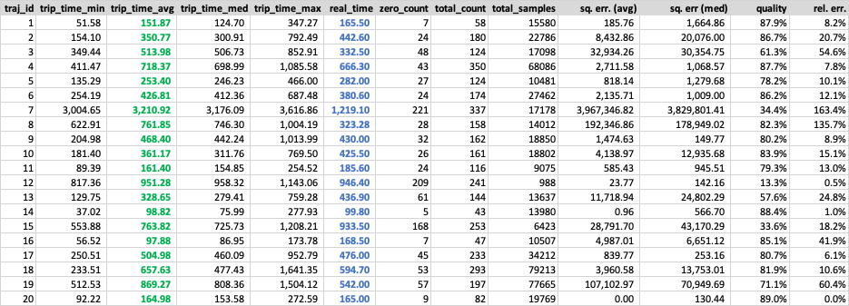
The output CSV file contains columns with the computed estimates for the trip time, including the minimum, average, median, and maximum times. These statistics deserve an explanation. The algorithm computes the average time using the average of each edge time distribution. It uses the same process to calculate the median. The minimum and maximum values derive from the limits of a two-sigma range, ensuring that the minimum value never goes below zero. The maximum is 𝜇+2𝜎, and the minimum is 𝜇-2𝜎 provided that this value is positive. When negative, the algorithm replaces it with the minimum value of the time range.
In the image above, the column with the prediction calculated using the average is green, while the column with the actual times is blue. To the right of it are three columns that help assess the quality of the underlying data. The first column counts the number of trip edges with no time data. You can compare it to the next column, which contains the number of queried edges for that trip. The ratio is in the "quality" computed column to the right. Lower values of this metric, such as in rows 7 and 12, reflect the lack of edge traversal time data. The final column contains the absolute relative error (computed against the average). Values in this column tend to have extreme values that negatively correlate to the data quality values, but this is just a hint.
By the very nature of this algorithm, the more data, the better it should predict trip times.
Conclusion
In this article, I presented a data-based alternative to improve the trip duration predictions of digital map service providers using a telematics database and map matching. The principle behind this solution is using a telematics database with data from the vehicles we want to model and their existing time distributions to project a planned trip.
This data-intensive process requires the collection of several samples of travel times between the most essential elements of a digital map: the edges between each node. We alleviate the search process using H3 indices, enabling simple indexation techniques.
The quality of the prediction will depend a lot on how adequate the data is for this process. We expect the best results with telematics databases from fleets with repeatable and stable routes.
Future Work
One of the areas for improvement of this prediction method is the data availability from past telematics. If you run a fleet that travels through repeated trajectories, data will be OK, but this might be an issue if your routes are more varied.
A possible line of research would be to find a way to extrapolate known time distributions to other road network edges with missing or insufficient data. Can we derive similarity measures between edges, or groups of edges, within the same road network? If so, and in case of missing data, we could use time distributions from other similar edges in the network to calculate the time prediction.
Another area that deserves some attention is the nature of the time distributions. This article assumes that no other factors impact the time distributions, which is likely untrue. We all know that traffic times vary throughout the day and week (to mention just two cycles). We should expect better results by studying and incorporating these behaviors into the predictions.
Finally, it would be very valuable for future development to include a provision for conditioning the edge time distributions along parameters such as the vehicle type, driver profile, or other relevant parameters. The algorithm would better predict trip times for the relevant conditions through conditioning and abundant data.
Licensing Information
The Extended Vehicle Energy Dataset is licensed under Apache 2.0, like its originator, the Vehicle Energy Dataset.
Reference Material
joaofig/eved-explore: An exploration of the Extended Vehicle Energy Dataset (github.com)
João Paulo Figueira is a Data Scientist at tb.lx by Daimler Truck in Lisbon, Portugal.
Map-Matching for Speed Prediction was originally published in Towards Data Science on Medium, where people are continuing the conversation by highlighting and responding to this story.
How fast will you drive?

When planning future vehicle routes, you trust the digital map providers for accurate speed predictions. You do this when picking your phone up to prepare for a car trip or, in a professional setting, when planning routes for your vehicle fleet. The forecasted speeds are an essential component of the trip’s cost, especially as they are one of the fundamental drivers of energy consumption in electric and combustion vehicles.
The digital mapping service providers collect information from live traffic and historical records to estimate how fast you can drive along a specific road at any given time. With this data and intelligent algorithms, they estimate how quickly an average vehicle will travel through the planned route. Some services will accept each vehicle’s features to tune the route path and the expected trip times.
But what about specific vehicles and drivers like yours? Do these predictions apply? Your cars and drivers might have particular requirements or habits that do not fit the standardized forecasts. Can we do better than the digital map service providers? We have a chance if you keep a good record of your historical telematics data.
Introduction
In this article, we will improve the quality of speed predictions from digital map providers by leveraging the historical speed profiles from a telematics database. This database contains records of past trips that we use to modulate the standard speed inferences from a digital map provider.
Central to this is map-matching, the process by which we “snap” the observed GPS locations to the underlying digital map. This correcting step allows us to bring the GPS measurements in line with the map’s road network representation, thus making all location sources comparable.
The Road Network
A road network is a mathematical concept that supports most digital mapping applications. Usually implemented as a directed multi-graph, each node represents a known geospatial location, usually some noteworthy landmark such as an intersection or a defining point on a road bend, and the connecting directed edges represent straight-line paths along the road. Figure 1 below illustrates the concept.
When we request a route from a digital map provider, we get a sequence of road network nodes and their connecting edges. The service also provides the estimated travel times and corresponding speeds between all pairs of nodes (in some cases, the speed estimates cover a range of nodes). We get the total trip duration by adding all the partial times together.
If we get better estimates for these times, we will also have better speed estimates and a better route prediction overall. The source for these better estimates is your historical telematics data. But knowing the historic speeds is just a part of the process. Before we can use these speeds, we must make sure that we can project them onto the digital map, and for this, we use map-matching.
Map-Matching
Map-matching projects sequences of GPS coordinates sampled from a moving object’s path to an existing road graph. The matching process uses a Hidden Markov Model to map the sampled locations to the most likely graph edge sequence. As a result, this process produces both the edge projections and the implicit node sequence. You can read a more detailed explanation in my previous article on map matching:
Map-Matching for Trajectory Prediction
After reading the above article, you will understand that the Valhalla map-matching algorithm projects the sampled GPS locations into road network edges, not to the nodes. The service may also return the matched poly-line defined in terms of the road network nodes. So, we can get both edge projections and the implicit node sequence.
On the other hand, when retrieving a route plan from the same provider, we also get a sequence of road network nodes. By matching these nodes to the previously map-matched ones, we can overlay the known telematics information to the newly generated route and thus improve the time and speed estimates with actual data.
Before using the map-matched locations to infer actual speeds, we must project them to the nodes and adjust the known travel times, as illustrated in Figure 2 below.
As a prerequisite, we must correctly sequence both sets of locations, the nodes, and the map matches. This process is depicted in Figure 2 above, where the map matches, represented by the orange diamonds, are sequenced along with the road network nodes, represented as red dots. The travel sequence is obviously from left to right.
We assume the time differences between the GPS locations are the same as the map-matched ones. This assumption, illustrated by Figure 3 below, is essential because there is no way to infer what effect in time the map matching has. This assumption simplifies the calculation while keeping a good approximation.
Now that we know the time differences between consecutive orange diamonds, our challenge is to use this information to infer the time differences between consecutive red dots (nodes). Figure 4 below shows the relationship between the two sequences of time differences.
We can safely assume that the average speeds between consecutive orange diamonds are constant. This assumption is essential for what comes next. But before we proceed, let’s define some terminology. We will use some simplifications due to Medium’s typesetting limitations.
We need to deal with two fundamental quantities: distances and timespans. Using Figure 4 above as a reference, we define the distance between the orange diamond one and red dot one as d(n1, m1). Here, the letter “m” stands for “map-matched,” and the letter “n” stands for node. Similarly, the corresponding timespan is t(n1, m1), and the average speed is v(n1, m1).
Let us focus on the first two nodes and see how we can derive the average speed (and the corresponding timespan) using the known timespans from orange diamonds one to four. The average speed of travel between the first two map-matched locations is thus:
Because the average speed is constant, we can now compute the first timespan.
The second timespan is just t(m2, m3). For the final period, we can repeat the process above. The total time is thus:
We must repeat this process, adapting it to the sequence of nodes and map matches to calculate the projected trip times between all nodes.
Now that we have seen how to project measured speeds onto a digital map let’s see where to get the data.
Telematics Database
This article uses a telematics database to infer unknown road segment average speeds. All the geospatial data in the database is already map-matched to the underlying digital map. This characteristic helps us match future service-provided routes to the known or projected road segment speeds using the abovementioned process.
Here, we will use a tried-and-true open-source telematics database I have been exploring lately and presented in a previously published article, the Extended Vehicle Energy Dataset (EVED), licensed under Apache 2.0.
Travel Time Estimation Using Quadkeys
Proposed Solution
We develop the solution in two steps: data preparation and prediction. In the data preparation step, we traverse all known trips in the telematics database and project the measured trip times to the corresponding road network edges. These computed edge traversal times are then stored in another database using maximum resolution H3 indices for faster searches during exploration. At the end of the process, we have collected traversal time distributions for the known edges, information that will allow us to estimate travel speeds in the prediction phase.
The prediction phase requires a source route expressed as a sequence of road network nodes, such as what we get from the Valhalla route planner. We query each pair of consecutive nodes' corresponding traversal time distribution (if any) from the speed database and use its mean (or median) to estimate the local average speed. By adding all edge estimates, we get the intended result, the expected total trip time.
Data Preparation
To prepare the data and generate the reference time distribution database, we must iterate through all the trips in the source data. Fortunately, the source database makes this easy by readily identifying all the trips (see the article above).
Let us look at the code that prepares the edge traversal times.
https://medium.com/media/d248980cdb01797aebfd16932fc03594/href
The code in Figure 5 above shows the main loop of the data preparation code. We use the previously created EVED database and save the output data to a new speed database. Each record is a time traversal sample for a single road network edge. For the same edge, a set of these samples makes up for a statistical time distribution, for which we calculate the average, median, and other statistics.
The call on line 5 retrieves a list of all the known trips in the source database as triplets containing the trajectory identifier (the table sequential identifier), the vehicle identifier, and the trip identifier. We need these last two items to retrieve the trip’s signals, as shown in line 10.
Lines 10 to 16 contain the code that retrieves the trip’s trajectory as a sequence of latitude, longitude, and timestamps. These locations do not necessarily correspond to road network nodes; they will mostly be projections into the edges (the orange diamonds in Figure 2).
Now, we can ask the Valhalla map-matching engine to take these points and return a poly-line with the corresponding road network node sequence, as shown in lines 18 to 25. These are the nodes that we store in the database, along with the projected traversal times, which we derive in the final lines of the code.
The traversal time projection from the map-matched locations to the node locations occurs in two steps. First, line 27 creates a “compound trajectory” object that merges the map-matched locations and the corresponding nodes in the trip sequence. The object stores each map-matched segment separately for later joining. Figure 6 below shows the object constructor (source file).
https://medium.com/media/20f2edca46fc9ab2acc9863324a535eb/href
The compound trajectory constructor starts by merging the sequence of map-matched points to the corresponding road network nodes. Referring to the symbols in Figure 2 above, the code combines the orange diamond sequence with the red dot sequence so they keep the trip order. In the first step, listed in Figure 7 below, we create a list of sequences of orange diamond pairs with any red dots in between.
https://medium.com/media/0b161ec19e1792caea41fc48dcadd0c4/href
Once merged, we convert the trajectory segments to node-based trajectories, removing the map-matched endpoints and recomputing the traversal times. Figure 8 below shows the function that computes the equivalent between-node traversal times.
https://medium.com/media/bfaae00ea29cf906f1132bb6b53c5396/href
Using the symbology of Figure 2, the code above uses the traversal times between two orange diamonds and calculates the times for all sub-segment traversals, namely between node-delimited ones. This way, we can later reconstruct all between-node traversal times through simple addition.
The final conversion step occurs on line 28 of Figure 5 when we convert the compound trajectory to a simple trajectory using the functions listed in Figure 9 below.
https://medium.com/media/1a614affe3d7a5f0155541949c36437a/href
The final step of the code in Figure 5 (lines 30–32) is to save the computed edge traversal times to the database for posterior use.
Data Quality
How good is the data that we just prepared? Does the EVED allow for good speed predictions? Unfortunately, this database was not designed for this purpose so that we will see some issues.
The first issue is the number of single-edge records in the final database, in this case, a little over two million. The total number of rows is over 5.6 million, so the unusable single-edge records represent a sizable proportion of the database. Almost half the rows are from edges with ten or fewer records.
The second issue is trips with very low frequencies. When querying an ad-hoc trip, we may fall into areas of very low density, where edge time records are scarce or nonexistent. In such conditions, the prediction code tries to compensate for the data loss using a simple heuristic: assume the same average speed as in the last edge. For larger road sections, and as we see below, we may even copy the data from the Valhalla route predictor.
The bottom line is that some of these predictions will be bad. A better use case for this algorithm would be to use a telematics database from fleets that frequently travel through the same routes. It would be even better to get more data for the same routes.
Prediction
To explore this time-prediction enhancement algorithm, we will use two different scripts: one interactive Streamlit application that allows you to freely use the map and an analytics script that tries to assess the quality of the predicted times by comparing them to known trip times in a LOOCV type of approach.
Interactive Map
You run the interactive application by executing the following command line at the project root:
streamlit run speed-predict.py
The interactive application allows you to specify endpoints of a route for Valhalla to predict. Figure 10 below shows what the user interface looks like.
To operate the application, use the drawing button below the zoom control to select the source, destination, and optional waypoints. The application draws the sequence as a blue line, as depicted. Next, press the “Predict” button on the top left, under the title. The application calls the Valhalla route predictor and draws its result as a red line. To the left, you see some of the output, namely the time estimates of the map provider and the two below from the algorithm described here. The first estimate uses the average of the matching edge time distributions, and the second uses the median. For missing data, the algorithm uses the map estimate.
Note that the application draws a black rectangle around the area where data is available. Outside of that area, all predictions will be the same as the map’s.
Accuracy Estimator
To estimate the accuracy of this time predictor, we will test it against known trips taken from the database. We will match the edge projections to the corresponding map nodes for each sampled trip and then query their duration distributions, excluding the data from the trip we want to estimate. This is a process akin to the known Leave-One-Out Cross Validation process.
Use the following command line to invoke the accuracy estimator script:
python benchmark-trips.py
When finished, the script outputs the estimates to a CSV file that you can use for accuracy analysis, as illustrated in Figure 11 below.
The output CSV file contains columns with the computed estimates for the trip time, including the minimum, average, median, and maximum times. These statistics deserve an explanation. The algorithm computes the average time using the average of each edge time distribution. It uses the same process to calculate the median. The minimum and maximum values derive from the limits of a two-sigma range, ensuring that the minimum value never goes below zero. The maximum is 𝜇+2𝜎, and the minimum is 𝜇-2𝜎 provided that this value is positive. When negative, the algorithm replaces it with the minimum value of the time range.
In the image above, the column with the prediction calculated using the average is green, while the column with the actual times is blue. To the right of it are three columns that help assess the quality of the underlying data. The first column counts the number of trip edges with no time data. You can compare it to the next column, which contains the number of queried edges for that trip. The ratio is in the "quality" computed column to the right. Lower values of this metric, such as in rows 7 and 12, reflect the lack of edge traversal time data. The final column contains the absolute relative error (computed against the average). Values in this column tend to have extreme values that negatively correlate to the data quality values, but this is just a hint.
By the very nature of this algorithm, the more data, the better it should predict trip times.
Conclusion
In this article, I presented a data-based alternative to improve the trip duration predictions of digital map service providers using a telematics database and map matching. The principle behind this solution is using a telematics database with data from the vehicles we want to model and their existing time distributions to project a planned trip.
This data-intensive process requires the collection of several samples of travel times between the most essential elements of a digital map: the edges between each node. We alleviate the search process using H3 indices, enabling simple indexation techniques.
The quality of the prediction will depend a lot on how adequate the data is for this process. We expect the best results with telematics databases from fleets with repeatable and stable routes.
Future Work
One of the areas for improvement of this prediction method is the data availability from past telematics. If you run a fleet that travels through repeated trajectories, data will be OK, but this might be an issue if your routes are more varied.
A possible line of research would be to find a way to extrapolate known time distributions to other road network edges with missing or insufficient data. Can we derive similarity measures between edges, or groups of edges, within the same road network? If so, and in case of missing data, we could use time distributions from other similar edges in the network to calculate the time prediction.
Another area that deserves some attention is the nature of the time distributions. This article assumes that no other factors impact the time distributions, which is likely untrue. We all know that traffic times vary throughout the day and week (to mention just two cycles). We should expect better results by studying and incorporating these behaviors into the predictions.
Finally, it would be very valuable for future development to include a provision for conditioning the edge time distributions along parameters such as the vehicle type, driver profile, or other relevant parameters. The algorithm would better predict trip times for the relevant conditions through conditioning and abundant data.
Licensing Information
The Extended Vehicle Energy Dataset is licensed under Apache 2.0, like its originator, the Vehicle Energy Dataset.
Reference Material
joaofig/eved-explore: An exploration of the Extended Vehicle Energy Dataset (github.com)
João Paulo Figueira is a Data Scientist at tb.lx by Daimler Truck in Lisbon, Portugal.
Map-Matching for Speed Prediction was originally published in Towards Data Science on Medium, where people are continuing the conversation by highlighting and responding to this story.
Denial of responsibility! Techno Blender is an automatic aggregator of the all world’s media. In each content, the hyperlink to the primary source is specified. All trademarks belong to their rightful owners, all materials to their authors. If you are the owner of the content and do not want us to publish your materials, please contact us by email – [email protected]. The content will be deleted within 24 hours.