Midimax Compression for Large Time-Series Data | by Edwin Sutrisno

Lightweight and fast compression algorithm in Python for time-series plots

Motivation

Visualization is a powerful and critical step for reasoning with our data. Plotting large time-series data however generates heavy file sizes which slow down user interaction and strain computing resources such as RAM, disk, network and more. In my line of work, time-series data from machinery monitoring sensors may be recorded at rates from 1 Hz (1 point per second) to thousands of Hz, easily generating 100k+ points per sensor per day and millions within a few days. In addition to the challenge of data length, plots typically need multiple variables in order to observe correlations thus exacerbating the resource constraint.

This article introduces a data compression algorithm called “Midimax” that is specifically geared to improve the performance of time-series plots through data size reduction. The name represents the underlying method of taking the minimum, median, and maximum points of windows split out of the original time-series data. The Midimax algorithm was developed with these 3 objectives in mind:

1. It should not introduce non-actual data. That means only return a subset of the original data, so no averaging, median interpolation, regression, and statistical aggregation. There are benefits in avoiding statistical manipulations on the underlying data when plotting, but we will not discuss them here.
2. It has to be fast and computationally light. It has to run on consumer computers and laptops. Ideally it should process 100k points in less than 3 seconds hence permitting scale-ups to longer data and more variables.
3. It should maximize information gain. That means it should capture variations in the original data as much as possible. This is where the minimum and maximum points are needed.
4. (Related to Point 3) Since taking the minimum and maximum points alone may give a false view of exaggerated variance, a median point is taken to retain an information about signal stability.

How It Works

To understand how Midimax works, here is a pseudo code:

1. Input to the algorithm a time-series data (e.g. Python Pandas Series) and a compression factor (float number).
2. Split the time-series data into non-overlapping windows of equal size where the size is calculated as: window_size = floor(3 * compression factor). The 3 is for the minimum, median, and maximum points taken from each window. So, to achieve a compression factor of 2, the window size has to be 6. Larger factors will require wider windows.
3. Sort the values in each window in ascending order.
4. Pick the first and last values for the min and max points. This will ensure we maximize the variance and retain information.
5. Pick a middle value for the median where the middle position is defined as med_index = floor(window_size/2). So, no interpolation is done even if the window size is even. In Python, index starts from 0.
6. Re-sort the picked points by the original index which is the timestamp.

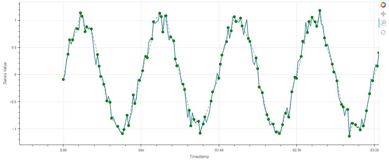
Example in Figure 1 below shows an original data (blue line) with 1 second sampling rate and the compression output (green dots) with a factor of 2. That means there are 50% less points after compression, so at the 50s mark there are only 25 green dots.

Full Code

The full code written in Python is available from GitHub.

Performance

A performance test was done to generate Bokeh plots of simulated time-series data with 1 million points. As a reference for benchmarking, the computing environment setup for testing is: Windows 10 64-bit laptop with 16 GB RAM, SSD disk, Intel Core i5 1.7 GHz processor, Python 3.7.10, Pandas 0.25.1, and Bokeh 2.3.2.

Input data was generated out of a sine wave plus Gaussian noise with 100,000 data points and saved as a Pandas Series before being passed into the compression function. A beginning part of the data is plotted in Figure 1 above.

A Python code to demonstrate the plotting performance is in the following:

import time
import numpy as np
import pandas as pdn = 100000 # points
timesteps = pd.to_timedelta(np.arange(n), unit=’s’)
timestamps = pd.to_datetime(“2022–04–18 08:00:00”) + timestepssine_waves = np.sin(2 * np.pi * 0.02 * np.arange(n))
noise = np.random.normal(0, 0.1, n)
signal = sine_waves + noise
ts_data = pd.Series(signal, index=timestamps).astype(‘float32’)# Run compression
timer_start = time.time()
ts_data_compressed = compress_series(ts_data, 2)
timer_sec = round(time.time() — timer_start, 2)
print(‘Compression took’, timer_sec, ‘seconds.’)> Compression took 0.45 seconds.

As shown in the code snippet above, the algorithm finished compressing 100k points by a factor of 2 in 1.42 seconds. Higher compression factors would finish faster because of less number of windows to process. Running compression factors of 4 and 8 on the same data completed in 0.74 s and 0.44 s respectively. Compressing 1 million points by factor 2 completed in 14.87 s.

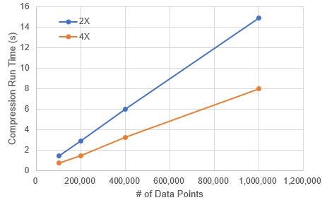
Figure 2 plots the algorithm run time for different compression factors and data sizes. we can observe that the run time grows linearly with the number of data points. This linear behavior allows predictability in performance when the application is scaled up.

Another metric to measure performance is the final file size of the plot. A Bokeh plot HTML file size for 1 million points is 15.6 MB before and 7.8 MB after a 2X compression.

Practical Usage Guide

In Figure 1 we can see that a compression factor of 2 resulted in a decent reconstruction of the original patterns. The quality of signal reconstruction is highly dependent on the original sampling rate of the data. If the original data was not adequately sampled then the compression would only worsen the final quality. It is advisable for the user to first try with different compression factors on a subset of data to find the right balance between size reduction and loss of fine details.

The Midimax algorithm was intended to improve visual performance, not for aiding modeling with large data. Although the algorithm offers a compression with good trend reconstruction, the distribution of the output data is vastly changed from the original. Using it for further analyses must be carefully thought.

Conclusion

Midimax is a simple and lightweight algorithm to reduce data size so that large time-series plots can be fast while consuming less computing resources. As with any compression method, details will be lost, but in the case of visual analysis, users are more interested in observing the general trends rather than small noises. The algorithm was demonstrated to capture the variations in the original data using a smaller number of points and to process large data within seconds.

GitHub repository: https://github.com/edwinsutrisno/midimax_compression

Lightweight and fast compression algorithm in Python for time-series plots

Motivation

Visualization is a powerful and critical step for reasoning with our data. Plotting large time-series data however generates heavy file sizes which slow down user interaction and strain computing resources such as RAM, disk, network and more. In my line of work, time-series data from machinery monitoring sensors may be recorded at rates from 1 Hz (1 point per second) to thousands of Hz, easily generating 100k+ points per sensor per day and millions within a few days. In addition to the challenge of data length, plots typically need multiple variables in order to observe correlations thus exacerbating the resource constraint.

This article introduces a data compression algorithm called “Midimax” that is specifically geared to improve the performance of time-series plots through data size reduction. The name represents the underlying method of taking the minimum, median, and maximum points of windows split out of the original time-series data. The Midimax algorithm was developed with these 3 objectives in mind:

1. It should not introduce non-actual data. That means only return a subset of the original data, so no averaging, median interpolation, regression, and statistical aggregation. There are benefits in avoiding statistical manipulations on the underlying data when plotting, but we will not discuss them here.
2. It has to be fast and computationally light. It has to run on consumer computers and laptops. Ideally it should process 100k points in less than 3 seconds hence permitting scale-ups to longer data and more variables.
3. It should maximize information gain. That means it should capture variations in the original data as much as possible. This is where the minimum and maximum points are needed.
4. (Related to Point 3) Since taking the minimum and maximum points alone may give a false view of exaggerated variance, a median point is taken to retain an information about signal stability.

How It Works

To understand how Midimax works, here is a pseudo code:

1. Input to the algorithm a time-series data (e.g. Python Pandas Series) and a compression factor (float number).
2. Split the time-series data into non-overlapping windows of equal size where the size is calculated as: window_size = floor(3 * compression factor). The 3 is for the minimum, median, and maximum points taken from each window. So, to achieve a compression factor of 2, the window size has to be 6. Larger factors will require wider windows.
3. Sort the values in each window in ascending order.
4. Pick the first and last values for the min and max points. This will ensure we maximize the variance and retain information.
5. Pick a middle value for the median where the middle position is defined as med_index = floor(window_size/2). So, no interpolation is done even if the window size is even. In Python, index starts from 0.
6. Re-sort the picked points by the original index which is the timestamp.

Example in Figure 1 below shows an original data (blue line) with 1 second sampling rate and the compression output (green dots) with a factor of 2. That means there are 50% less points after compression, so at the 50s mark there are only 25 green dots.

Full Code

The full code written in Python is available from GitHub.

Performance

A performance test was done to generate Bokeh plots of simulated time-series data with 1 million points. As a reference for benchmarking, the computing environment setup for testing is: Windows 10 64-bit laptop with 16 GB RAM, SSD disk, Intel Core i5 1.7 GHz processor, Python 3.7.10, Pandas 0.25.1, and Bokeh 2.3.2.

Input data was generated out of a sine wave plus Gaussian noise with 100,000 data points and saved as a Pandas Series before being passed into the compression function. A beginning part of the data is plotted in Figure 1 above.

A Python code to demonstrate the plotting performance is in the following:

import time
import numpy as np
import pandas as pdn = 100000 # points
timesteps = pd.to_timedelta(np.arange(n), unit=’s’)
timestamps = pd.to_datetime(“2022–04–18 08:00:00”) + timestepssine_waves = np.sin(2 * np.pi * 0.02 * np.arange(n))
noise = np.random.normal(0, 0.1, n)
signal = sine_waves + noise
ts_data = pd.Series(signal, index=timestamps).astype(‘float32’)# Run compression
timer_start = time.time()
ts_data_compressed = compress_series(ts_data, 2)
timer_sec = round(time.time() — timer_start, 2)
print(‘Compression took’, timer_sec, ‘seconds.’)> Compression took 0.45 seconds.

As shown in the code snippet above, the algorithm finished compressing 100k points by a factor of 2 in 1.42 seconds. Higher compression factors would finish faster because of less number of windows to process. Running compression factors of 4 and 8 on the same data completed in 0.74 s and 0.44 s respectively. Compressing 1 million points by factor 2 completed in 14.87 s.

Figure 2 plots the algorithm run time for different compression factors and data sizes. we can observe that the run time grows linearly with the number of data points. This linear behavior allows predictability in performance when the application is scaled up.

Another metric to measure performance is the final file size of the plot. A Bokeh plot HTML file size for 1 million points is 15.6 MB before and 7.8 MB after a 2X compression.

Practical Usage Guide

In Figure 1 we can see that a compression factor of 2 resulted in a decent reconstruction of the original patterns. The quality of signal reconstruction is highly dependent on the original sampling rate of the data. If the original data was not adequately sampled then the compression would only worsen the final quality. It is advisable for the user to first try with different compression factors on a subset of data to find the right balance between size reduction and loss of fine details.

The Midimax algorithm was intended to improve visual performance, not for aiding modeling with large data. Although the algorithm offers a compression with good trend reconstruction, the distribution of the output data is vastly changed from the original. Using it for further analyses must be carefully thought.

Conclusion

Midimax is a simple and lightweight algorithm to reduce data size so that large time-series plots can be fast while consuming less computing resources. As with any compression method, details will be lost, but in the case of visual analysis, users are more interested in observing the general trends rather than small noises. The algorithm was demonstrated to capture the variations in the original data using a smaller number of points and to process large data within seconds.

GitHub repository: https://github.com/edwinsutrisno/midimax_compression