Modeling the Traveling Salesman Problem from first principles

A concepts-first, math-second approach to modeling the most well-known routing problem in Operations Research

👁️ This is article #2 of the series covering the project “An Intelligent Decision Support System for Tourism in Python”. I encourage you to check it out to get a general overview of the whole project. If you’re only interested in how to model the TSP, you’re still at the right place, as this article is self-contained. If you’re also interested in solving the problem, not just modeling it, you’ll love the next 5 articles of the series. Trust me, they’ll provide you with what you need and what you didn’t know you needed 😉

Table of contents

1. Motivation and purpose

2. Understanding the data

3. Defining a conceptual model from the problem description

4. Building a mathematical model from the conceptual model

• 4.1. Putting the data in Sets and Parameters
• 4.2. Encoding decisions in Variables
• 4.3. Defining the Objective
• 4.4. Creating the Constraints

1. Motivation and purpose

This article continues right where the article for sprint 1 left off. You don’t need to have read it to understand what we’ll do here, but let me give you a quick recap (feel free to jump to section 2 if you did read the previous article). In a nutshell, we laid out the common problems that tourists face when planning a trip, and we set out to build a system that can help us plan trips more effectively, speeding up decision-making, or even fully automating the schedule for any given trip. We observed that stated like that, the problem is too complex, so we decomposed it and arrived at its essential version, and we called it the minimum valuable problem. In the end, we concluded that it took the form of the Traveling Salesman Problem (TSP), where the “cities” that the proverbial salesman must visit correspond, in our version, to the “sites of interest” in a city that a tourist desires to visit.

So, as a kickstarter, we must first formulate and solve the TSP, and once that’s done, we’ll be on firm grounds to progress toward a more sophisticated and general solution to our trip planning problem. We chose this approach because this article series also teaches an agile approach to modeling in Operations Research (OR), so many of the lessons, tips, and tricks you’ll find here are applicable to any kind of problem you may face in OR in general.

Returning to our business, we have the problem description of the TSP:

• Goal: walk as little distance as possible
• Requirements: visit each site only once, and return to the original departure site (in our case, the hotel).

Since we know that this problem is not our real problem, but a simple approximation to it, we want to build a model of the problem, as a model can be refined, augmented, and tweaked; and we know we’ll need to do that to arrive at a solution to our real problem. Hence, our goal is to build a model, as opposed to finding a direct solution to it or devising some kind of heuristic algorithm that finds some solution for you. Once you learn how to reason your way into such a model, you will have a good understanding to go and read the next sprint’s article, where we will implement the model in Python.

2. Understanding the data

If you recall from our last sprint, the basic input for the TSP is just a list of sites that we want to visit in a single day. In this proof-of-concept, we’re using Paris, so I’ve chosen these eight famous, must-visit places:

• Sacre Coeur
• Louvre
• Montmartre
• Port de Suffren
• Arc de Triomphe
• Av. Champs Élysées
• Notre Dame
• Tour Eiffel

Since the problem consists of finding a tour of minimal distance, the actual data we need is distance data, which depends on the sites and their relative geographic positions. How to compute distance data from geographic locations will be covered in sprint 4, since covering it now would entail a de-tour (pun intended) that would distract you from the main focus here: model building.

So, for now, consider you’re given the distances between all possible pairs. They will be given as a CSV file in the next sprint when we implement the model in Python. The data looks like this:

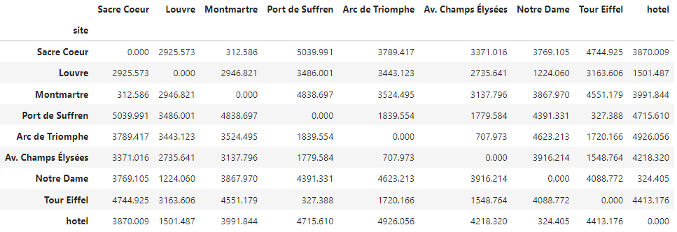
We’ll call this table the distance matrix. Note that, although not particularly postcard-worthy, the hotel is included in the matrix too, as it counts as another site that needs to be in the final tour. For this MVP, we keep things simple and use a symmetric distance matrix, which is a fancy way of saying that the distance from 𝐴 to 𝐵 is the same as the distance from 𝐵 to 𝐴, for any A and B. In more advanced settings, this need not be the case to a relevant degree, making this approximation ineffective.

3. Defining a conceptual model from the problem description

Now we’re at the stage represented as the green block in the flowchart below:

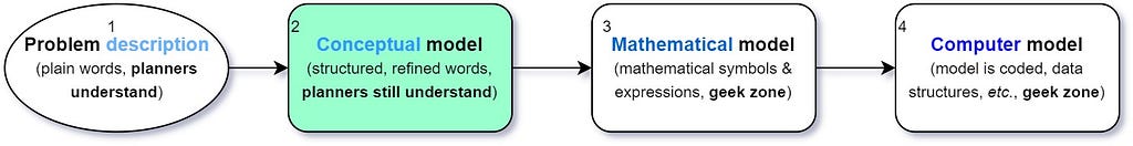
The purpose of the conceptual model is to state the problem using words, but in a standardized format, so that the mapping between “sentences” and “mathematical objects” becomes clear later in the subsequent phase (mathematical model formulation). We can postulate our conceptual model like this:

(Knowing)

Data (sets and parameters):

• The list of sites to visit
• The distance between any pair of sites

(We need to decide)

Decisions: In which order to visit the sites

(In a way that we)

Objective: Minimize the total distance traveled

(Such that)

Constraints:

• All sites are visited
• Each site is visited just once
• The last site visited is the site we started from (we do a closed tour)

👁️ Follow good practices and, in practice, goodness will follow you

You may have thought that the conceptual model looks quite trivial and not very different from the “simple” problem statement we started the article with. And you would be right. For small problems like this one, it can be a repetitive step. But for bigger problems, this stage is indispensable, and attempting to build a mathematical model without having a conceptual model first usually translates into mayhem (unclear or vague requirements, bad formulations, buggy code, infeasible models, etc.) Thus, it is paramount that we build the discipline now and go through this stage here too, even if the marginal value in our simple case is very low. Focus on good habits, and good results will follow.

4. Building a mathematical model from the conceptual model

We just reached “stage 3” of the workflow, in green below. The “mathematical model stage”, probably the most challenging stage of all, is where natural language becomes mathematics.

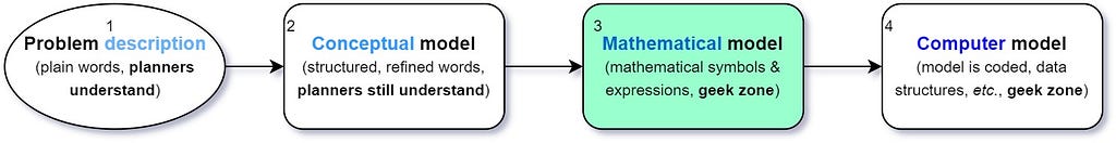
It is at this stage where not even the least amount of ambiguity is permitted.

A well defined mathematical model is worth a hundred clarifications

In this stage of our workflow, we build a pure model for the TSP, and in the next phase (covered in “sprint 3”) we will construct a model instance out of the CSV dataset we explained earlier, with the help of Python.

📝 Theory refresher: “abstract model” vs “model instance”

Mathematical models (in OR) are made of “components”. These are all the elements (equations, data, etc.) that collectively represent a problem of a certain structure. What truly defines a model is its structure, i.e., how its components relate to each other, regardless of the particular numerical values that these components take in any given example.

A model instance is a specific “materialization” of an “abstract model” with concrete data. Thus, we normally define abstract models, then populate them with data of particular scenarios, which yields model instances. It is those model instances that we optimize to get concrete results.

In the subsections below, I will briefly touch on the components that make up a model, and their purposes, while I’m defining them. Feel free to skip these explanations, and jump directly to the mathematical definitions, if you are not a beginner and already know the functions of the model components.

4.1. Putting the data in Sets and Parameters

All the data we need resides in the dataframe displayed in Figure 2.1. We could keep the data only there, fetching all the numbers from that dataframe when creating the constraints and objective of the model. In fact many people do that, but it’s a bad habit that doesn’t scale well with the size of the model. As the model complexity grows, this approach necessitates of ever growing glue code (to deal with dataframe operations) that could be avoided if the data were kept organized in other data structures more geared towards the building of optimization models. These data structures are the sets and parameters of a model.

💡 Different data structures to serve different needs

In case you were wondering “Why create sets and parameters, when we already have the data we need in a table?”, the short answer is: because doing so makes the model building easier, more general, and less error-prone.

“Sets” are the model components used to store the main “entities”, or “elements”, of a problem, whereas “parameters” are used to store the numerical properties of those entities, or of their relationships. In our example, the sites are the main “entities”, so they will be stored in a set, and the distances between pairs of sites are the “numerical properties” of their relationships, so they will be stored as parameters. At the “implementation level”, it is also very useful to make this categorization because each component serves a different function that will make model building easier:

• The function of sets is the convenient storage and manipulation of indices. These indices are the IDs or names that represent the different “entities” of the problem, and they are used to index parameters in convenient ways for the creation of constraints and objectives.

• The function of parameters is the convenient storage and manipulation of numerical properties of the “entities” they are indexed by, and these are the numbers that actually appear in the constraints and objectives.

From our conceptual model, we have:

• The list of sites to visit, which we define as the set 𝕊:

The phrase “indexed by 𝑖, 𝑗” is placed next to the set definition to signal that whenever the indices 𝑖 or 𝑗 are used in the model, they represent members of 𝕊. That way, when we have several sets, and thus multiple indices in use, it’s easier to remember what each index means.

• The distance between any pair of sites, which we define as the indexed parameter 𝐷ᵢⱼ:

The parameter is called “indexed” simply to indicate that it is not a scalar parameter (i.e., a single number), but a 2-D matrix of numbers. To retrieve a number from this indexed parameter you need to specify two indices, 𝑖 and 𝑗, which in turn will be taken from the set 𝕊.

𝕊 and 𝐷ᵢⱼ are the only “data components” present in the conceptual model. But that shouldn’t limit our ability to come up with other sets or parameters that prove useful when building a model.

As an illustration, note that the indices of 𝐷ᵢⱼ, 𝑖 and 𝑗, are members of 𝕊 but cannot coincide. If they did, the distance would be zero, which is a trivial datum. Besides, we would never go from one place to itself again, so it is useless to consider pairs (𝑖, 𝑖) at all. Thus, it’s useful to limit the combinations that pairs (𝑖, 𝑗) can take, so that modeling becomes easier (and errors less likely). To that end, we now create another set, 𝔸, derived from 𝕊, that contains all pairs (𝑖, 𝑗) of different sites. Each pair represents an arc connecting site 𝑖 to site 𝑗, hence the symbol 𝔸.

📝 An arc is just a “directed link” between two nodes of a “network”. Just think of an arc (𝑖, 𝑗) as a vector starting at 𝑖 and ending at 𝑗. When the “link” between two nodes is not directed (i.e., the direction is irrelevant) the word “edge” is used, as saying “undirected arc” all the time would be too wordy. People in Graph Theory like to be efficient too.

A nice property of 𝔸 is that it is the domain over which 𝐷ᵢⱼ is defined, and as we will see when implementing the model in Python, defining such a domain explicitly makes it reusable for other model components, and that’s also convenient.

• Set of possible arcs between different sites:

4.2. Encoding decisions in variables

Since we are building a model so it can tell us what actions we should take, and these prescribed actions are unknown to us before the model is optimized, we must encode into variables all the potential actions we could take.

But how do we define such potential actions? From our conceptual model, the generic “decision” we need to make is the “order in which to visit the sites”. This “order” refers to one path among all possible paths we could follow when doing a tour. The key idea is that a path is made of a sequence of arcs connecting individual nodes (i.e., sites). Therefore, deciding to do a particular path is actually deciding to traverse a particular sequence of arcs. These “atomic decisions” about whether or not to traverse a particular arc connecting two sites are the decisions we want to encode as variables.

“Whether or not to go from site A to site B” is clearly a binary decision: either I go, or I don’t. Because of this nature, the decision variables need to be binary (i.e., taking only 0 or 1 as values) and are defined only for valid arcs (for which the derived 𝔸 comes in handy now). In mathematical terms:

There is a unique decision variable for each possible arc (𝑖, 𝑗), but when the model is optimized, we will only be interested in the variables that take the value 1, for they indicate what arcs should be traversed. For example, if the variable 𝛿ᵢⱼ, with 𝑖=hotel, and 𝑗=Louvre, takes the value 1, it means we should go from the hotel to the Louvre as part of our tour.

4.3. Defining the objective

Imagine we have 4 points, 𝑎, 𝑏, 𝑐, 𝑑, and we follow the path 𝑎 → 𝑏 → 𝑐, in which point 𝑑 is not visited. Its total distance is the sum of the distances of its arcs: 𝐷ᵃᵇ + 𝐷ᵇᶜ. But, if we don’t know in advance what path we will follow, how do we represent the total distance of this unknown path?

💡 Precisely because the optimal path is unknown, we need an expression that covers all possible paths, but that reduces to the distance of the “best path” when the model is optimized.

By exploiting the fact that any traversed arc (𝑖, 𝑗) will have 𝛿ᵢⱼ = 1, and any untraversed arc (𝑖′,𝑗′) will have 𝛿ᵢᑊⱼᑊ = 0, we can create an expression that, once the variables have been decided, will reduce to the total distance of the traversed path. The way to do that is to “add up all potentialities”, i.e., to do the summation over all possible arc distances 𝐷ᵢⱼ weighted by their binary “arc variables” 𝛿ᵢⱼ, and let the 0’s and 1’s that those variables will take decide which distances remain (𝐷ᵢⱼ × 1 = 𝐷ᵢⱼ) and which vanish (𝐷ᵢⱼ × 0 = 0), in the expression for the total distance. This “summation of potentialities” represents the total distance the final tour will take, so it will be our objective (called 𝑍) to be minimized.

Mathematically, this is expressed as:

Note how the summation at the right has become simpler to read (and implement) thanks to the use of 𝔸, the domain (set of indices) for both 𝐷ᵢⱼ and 𝛿ᵢⱼ.

Also, note that the objective constitutes our definition of goodness. Since we want to minimize it, a lower value is better than a higher value, so obviously, the minimum value is the best value. The values of the decision variables 𝛿ᵢⱼ that correspond to this “best” value of the objective constitute the (optimal) solution to the problem, and they will be found by the optimization process.

4.4. Creating the constraints

From our conceptual model, we have:

1. All sites are visited.
2. Each site is visited just once
3. The last site visited is the site we started from (we do a closed tour)

We realize that requirement (1) is already “included” in requirement (2), for if each site is visited just once, that entails each site is visited, and thus all sites are visited. So we dismiss the need for a separate constraint for requirement (1) and focus on how to model requirement (2) as a constraint.

To say that “each site is visited just once” is the same as to say that “each site is entered and exited just once”. And that phrase, in turn, is equivalent to these two phrases together: “each site is entered just once” and “each site is exited just once”. Let’s model the “phrases” separately:

• Each site is entered just once:

It’s useful to read the whole expression from right to left. If you first see over which indices the constraint is defined, interpreting the meaning of the constraint definition on the left side will be easier. I would read this constraint aloud as:

for each site 𝑗 belonging to the set of all sites 𝕊, the sum of all potential arcs 𝛿ᵢⱼ arriving at 𝑗 must be equal to 1, meaning that only one incoming arc must happen at 𝑗. Or, more colloquially: each site must be visited from only one other site.

• Each site is exited just once:

I would read this constraint as:

for each site 𝑖 belonging to the set of all sites 𝕊, the sum of all potential arcs 𝛿ᵢⱼ departing from 𝑖 must be equal to 1, meaning that only one outgoing arc must happen at 𝑖. Or, more colloquially: each site must departure to only one other site.

We’re left with only requirement (3). It states that the optimal path must finish at the same site it started from, or equivalently, that the path must be a tour (a closed loop). Here’s a possible line of reasoning one can have at first sight: “Because we have already created constraints to enforce that each site is both entered and exited once, this implies that the resulting path must be closed, since it is impossible for any site to be a “sink” (i.e., a site has one incoming arc but no outgoing arcs) or to be a “source” (i.e., a site has an outgoing arc but no incoming arcs). Therefore, the previous two constraints, presumably, force the final trajectory to be a closed loop”.

Is that line of reasoning correct? Let’s take an experimental approach. Let’s assume this reasoning is correct, and try to solve the model as is now. When we look at the solution, we will see if it looks right or if something’s wrong. If the results are wrong (or don’t make sense in any way), we can always go back and revise our logic (something which in real-life projects happens all the time). The implementation, solution, and “experimental validation” is what it’s covered in our “next sprint”, where a Python model is created, solved, inspected, and re-formulated based on the results we get.

Thus, we conclude here (tentatively) the “mathematical model formulation” stage. Next stop: the “computer model implementation”, carried out in Implementing, solving, and visualizing the Traveling Salesman Problem with Python.

There will be more articles of more “sprints” coming out, so if you’re eager to be my companion on this journey, stay tuned and check the project timeline in section 3 of the first article in this series, to navigate to your desired sprint and follow the work being done there.

Also, feel free to follow me, ask me questions in the comments, give me feedback, or contact me on LinkedIn.

Thanks for reading, and see you in the next one! 📈😊

References:

• Wikipedia. The Traveling Salesman Problem

Modeling the Traveling Salesman Problem from first principles was originally published in Towards Data Science on Medium, where people are continuing the conversation by highlighting and responding to this story.

A concepts-first, math-second approach to modeling the most well-known routing problem in Operations Research

👁️ This is article #2 of the series covering the project “An Intelligent Decision Support System for Tourism in Python”. I encourage you to check it out to get a general overview of the whole project. If you’re only interested in how to model the TSP, you’re still at the right place, as this article is self-contained. If you’re also interested in solving the problem, not just modeling it, you’ll love the next 5 articles of the series. Trust me, they’ll provide you with what you need and what you didn’t know you needed 😉

Table of contents

1. Motivation and purpose

2. Understanding the data

3. Defining a conceptual model from the problem description

4. Building a mathematical model from the conceptual model

• 4.1. Putting the data in Sets and Parameters
• 4.2. Encoding decisions in Variables
• 4.3. Defining the Objective
• 4.4. Creating the Constraints

1. Motivation and purpose

This article continues right where the article for sprint 1 left off. You don’t need to have read it to understand what we’ll do here, but let me give you a quick recap (feel free to jump to section 2 if you did read the previous article). In a nutshell, we laid out the common problems that tourists face when planning a trip, and we set out to build a system that can help us plan trips more effectively, speeding up decision-making, or even fully automating the schedule for any given trip. We observed that stated like that, the problem is too complex, so we decomposed it and arrived at its essential version, and we called it the minimum valuable problem. In the end, we concluded that it took the form of the Traveling Salesman Problem (TSP), where the “cities” that the proverbial salesman must visit correspond, in our version, to the “sites of interest” in a city that a tourist desires to visit.

So, as a kickstarter, we must first formulate and solve the TSP, and once that’s done, we’ll be on firm grounds to progress toward a more sophisticated and general solution to our trip planning problem. We chose this approach because this article series also teaches an agile approach to modeling in Operations Research (OR), so many of the lessons, tips, and tricks you’ll find here are applicable to any kind of problem you may face in OR in general.

Returning to our business, we have the problem description of the TSP:

• Goal: walk as little distance as possible
• Requirements: visit each site only once, and return to the original departure site (in our case, the hotel).

Since we know that this problem is not our real problem, but a simple approximation to it, we want to build a model of the problem, as a model can be refined, augmented, and tweaked; and we know we’ll need to do that to arrive at a solution to our real problem. Hence, our goal is to build a model, as opposed to finding a direct solution to it or devising some kind of heuristic algorithm that finds some solution for you. Once you learn how to reason your way into such a model, you will have a good understanding to go and read the next sprint’s article, where we will implement the model in Python.

2. Understanding the data

If you recall from our last sprint, the basic input for the TSP is just a list of sites that we want to visit in a single day. In this proof-of-concept, we’re using Paris, so I’ve chosen these eight famous, must-visit places:

• Sacre Coeur
• Louvre
• Montmartre
• Port de Suffren
• Arc de Triomphe
• Av. Champs Élysées
• Notre Dame
• Tour Eiffel

Since the problem consists of finding a tour of minimal distance, the actual data we need is distance data, which depends on the sites and their relative geographic positions. How to compute distance data from geographic locations will be covered in sprint 4, since covering it now would entail a de-tour (pun intended) that would distract you from the main focus here: model building.

So, for now, consider you’re given the distances between all possible pairs. They will be given as a CSV file in the next sprint when we implement the model in Python. The data looks like this:

We’ll call this table the distance matrix. Note that, although not particularly postcard-worthy, the hotel is included in the matrix too, as it counts as another site that needs to be in the final tour. For this MVP, we keep things simple and use a symmetric distance matrix, which is a fancy way of saying that the distance from 𝐴 to 𝐵 is the same as the distance from 𝐵 to 𝐴, for any A and B. In more advanced settings, this need not be the case to a relevant degree, making this approximation ineffective.

3. Defining a conceptual model from the problem description

Now we’re at the stage represented as the green block in the flowchart below:

The purpose of the conceptual model is to state the problem using words, but in a standardized format, so that the mapping between “sentences” and “mathematical objects” becomes clear later in the subsequent phase (mathematical model formulation). We can postulate our conceptual model like this:

(Knowing)

Data (sets and parameters):

• The list of sites to visit
• The distance between any pair of sites

(We need to decide)

Decisions: In which order to visit the sites

(In a way that we)

Objective: Minimize the total distance traveled

(Such that)

Constraints:

• All sites are visited
• Each site is visited just once
• The last site visited is the site we started from (we do a closed tour)

👁️ Follow good practices and, in practice, goodness will follow you

You may have thought that the conceptual model looks quite trivial and not very different from the “simple” problem statement we started the article with. And you would be right. For small problems like this one, it can be a repetitive step. But for bigger problems, this stage is indispensable, and attempting to build a mathematical model without having a conceptual model first usually translates into mayhem (unclear or vague requirements, bad formulations, buggy code, infeasible models, etc.) Thus, it is paramount that we build the discipline now and go through this stage here too, even if the marginal value in our simple case is very low. Focus on good habits, and good results will follow.

4. Building a mathematical model from the conceptual model

We just reached “stage 3” of the workflow, in green below. The “mathematical model stage”, probably the most challenging stage of all, is where natural language becomes mathematics.

It is at this stage where not even the least amount of ambiguity is permitted.

A well defined mathematical model is worth a hundred clarifications

In this stage of our workflow, we build a pure model for the TSP, and in the next phase (covered in “sprint 3”) we will construct a model instance out of the CSV dataset we explained earlier, with the help of Python.

📝 Theory refresher: “abstract model” vs “model instance”

Mathematical models (in OR) are made of “components”. These are all the elements (equations, data, etc.) that collectively represent a problem of a certain structure. What truly defines a model is its structure, i.e., how its components relate to each other, regardless of the particular numerical values that these components take in any given example.

A model instance is a specific “materialization” of an “abstract model” with concrete data. Thus, we normally define abstract models, then populate them with data of particular scenarios, which yields model instances. It is those model instances that we optimize to get concrete results.

In the subsections below, I will briefly touch on the components that make up a model, and their purposes, while I’m defining them. Feel free to skip these explanations, and jump directly to the mathematical definitions, if you are not a beginner and already know the functions of the model components.

4.1. Putting the data in Sets and Parameters

All the data we need resides in the dataframe displayed in Figure 2.1. We could keep the data only there, fetching all the numbers from that dataframe when creating the constraints and objective of the model. In fact many people do that, but it’s a bad habit that doesn’t scale well with the size of the model. As the model complexity grows, this approach necessitates of ever growing glue code (to deal with dataframe operations) that could be avoided if the data were kept organized in other data structures more geared towards the building of optimization models. These data structures are the sets and parameters of a model.

💡 Different data structures to serve different needs

In case you were wondering “Why create sets and parameters, when we already have the data we need in a table?”, the short answer is: because doing so makes the model building easier, more general, and less error-prone.

“Sets” are the model components used to store the main “entities”, or “elements”, of a problem, whereas “parameters” are used to store the numerical properties of those entities, or of their relationships. In our example, the sites are the main “entities”, so they will be stored in a set, and the distances between pairs of sites are the “numerical properties” of their relationships, so they will be stored as parameters. At the “implementation level”, it is also very useful to make this categorization because each component serves a different function that will make model building easier:

• The function of sets is the convenient storage and manipulation of indices. These indices are the IDs or names that represent the different “entities” of the problem, and they are used to index parameters in convenient ways for the creation of constraints and objectives.

• The function of parameters is the convenient storage and manipulation of numerical properties of the “entities” they are indexed by, and these are the numbers that actually appear in the constraints and objectives.

From our conceptual model, we have:

• The list of sites to visit, which we define as the set 𝕊:

The phrase “indexed by 𝑖, 𝑗” is placed next to the set definition to signal that whenever the indices 𝑖 or 𝑗 are used in the model, they represent members of 𝕊. That way, when we have several sets, and thus multiple indices in use, it’s easier to remember what each index means.

• The distance between any pair of sites, which we define as the indexed parameter 𝐷ᵢⱼ:

The parameter is called “indexed” simply to indicate that it is not a scalar parameter (i.e., a single number), but a 2-D matrix of numbers. To retrieve a number from this indexed parameter you need to specify two indices, 𝑖 and 𝑗, which in turn will be taken from the set 𝕊.

𝕊 and 𝐷ᵢⱼ are the only “data components” present in the conceptual model. But that shouldn’t limit our ability to come up with other sets or parameters that prove useful when building a model.

As an illustration, note that the indices of 𝐷ᵢⱼ, 𝑖 and 𝑗, are members of 𝕊 but cannot coincide. If they did, the distance would be zero, which is a trivial datum. Besides, we would never go from one place to itself again, so it is useless to consider pairs (𝑖, 𝑖) at all. Thus, it’s useful to limit the combinations that pairs (𝑖, 𝑗) can take, so that modeling becomes easier (and errors less likely). To that end, we now create another set, 𝔸, derived from 𝕊, that contains all pairs (𝑖, 𝑗) of different sites. Each pair represents an arc connecting site 𝑖 to site 𝑗, hence the symbol 𝔸.

📝 An arc is just a “directed link” between two nodes of a “network”. Just think of an arc (𝑖, 𝑗) as a vector starting at 𝑖 and ending at 𝑗. When the “link” between two nodes is not directed (i.e., the direction is irrelevant) the word “edge” is used, as saying “undirected arc” all the time would be too wordy. People in Graph Theory like to be efficient too.

A nice property of 𝔸 is that it is the domain over which 𝐷ᵢⱼ is defined, and as we will see when implementing the model in Python, defining such a domain explicitly makes it reusable for other model components, and that’s also convenient.

• Set of possible arcs between different sites:

4.2. Encoding decisions in variables

Since we are building a model so it can tell us what actions we should take, and these prescribed actions are unknown to us before the model is optimized, we must encode into variables all the potential actions we could take.

But how do we define such potential actions? From our conceptual model, the generic “decision” we need to make is the “order in which to visit the sites”. This “order” refers to one path among all possible paths we could follow when doing a tour. The key idea is that a path is made of a sequence of arcs connecting individual nodes (i.e., sites). Therefore, deciding to do a particular path is actually deciding to traverse a particular sequence of arcs. These “atomic decisions” about whether or not to traverse a particular arc connecting two sites are the decisions we want to encode as variables.

“Whether or not to go from site A to site B” is clearly a binary decision: either I go, or I don’t. Because of this nature, the decision variables need to be binary (i.e., taking only 0 or 1 as values) and are defined only for valid arcs (for which the derived 𝔸 comes in handy now). In mathematical terms:

There is a unique decision variable for each possible arc (𝑖, 𝑗), but when the model is optimized, we will only be interested in the variables that take the value 1, for they indicate what arcs should be traversed. For example, if the variable 𝛿ᵢⱼ, with 𝑖=hotel, and 𝑗=Louvre, takes the value 1, it means we should go from the hotel to the Louvre as part of our tour.

4.3. Defining the objective

Imagine we have 4 points, 𝑎, 𝑏, 𝑐, 𝑑, and we follow the path 𝑎 → 𝑏 → 𝑐, in which point 𝑑 is not visited. Its total distance is the sum of the distances of its arcs: 𝐷ᵃᵇ + 𝐷ᵇᶜ. But, if we don’t know in advance what path we will follow, how do we represent the total distance of this unknown path?

💡 Precisely because the optimal path is unknown, we need an expression that covers all possible paths, but that reduces to the distance of the “best path” when the model is optimized.

By exploiting the fact that any traversed arc (𝑖, 𝑗) will have 𝛿ᵢⱼ = 1, and any untraversed arc (𝑖′,𝑗′) will have 𝛿ᵢᑊⱼᑊ = 0, we can create an expression that, once the variables have been decided, will reduce to the total distance of the traversed path. The way to do that is to “add up all potentialities”, i.e., to do the summation over all possible arc distances 𝐷ᵢⱼ weighted by their binary “arc variables” 𝛿ᵢⱼ, and let the 0’s and 1’s that those variables will take decide which distances remain (𝐷ᵢⱼ × 1 = 𝐷ᵢⱼ) and which vanish (𝐷ᵢⱼ × 0 = 0), in the expression for the total distance. This “summation of potentialities” represents the total distance the final tour will take, so it will be our objective (called 𝑍) to be minimized.

Mathematically, this is expressed as:

Note how the summation at the right has become simpler to read (and implement) thanks to the use of 𝔸, the domain (set of indices) for both 𝐷ᵢⱼ and 𝛿ᵢⱼ.

Also, note that the objective constitutes our definition of goodness. Since we want to minimize it, a lower value is better than a higher value, so obviously, the minimum value is the best value. The values of the decision variables 𝛿ᵢⱼ that correspond to this “best” value of the objective constitute the (optimal) solution to the problem, and they will be found by the optimization process.

4.4. Creating the constraints

From our conceptual model, we have:

1. All sites are visited.
2. Each site is visited just once
3. The last site visited is the site we started from (we do a closed tour)

We realize that requirement (1) is already “included” in requirement (2), for if each site is visited just once, that entails each site is visited, and thus all sites are visited. So we dismiss the need for a separate constraint for requirement (1) and focus on how to model requirement (2) as a constraint.

To say that “each site is visited just once” is the same as to say that “each site is entered and exited just once”. And that phrase, in turn, is equivalent to these two phrases together: “each site is entered just once” and “each site is exited just once”. Let’s model the “phrases” separately:

• Each site is entered just once:

It’s useful to read the whole expression from right to left. If you first see over which indices the constraint is defined, interpreting the meaning of the constraint definition on the left side will be easier. I would read this constraint aloud as:

for each site 𝑗 belonging to the set of all sites 𝕊, the sum of all potential arcs 𝛿ᵢⱼ arriving at 𝑗 must be equal to 1, meaning that only one incoming arc must happen at 𝑗. Or, more colloquially: each site must be visited from only one other site.

• Each site is exited just once:

I would read this constraint as:

for each site 𝑖 belonging to the set of all sites 𝕊, the sum of all potential arcs 𝛿ᵢⱼ departing from 𝑖 must be equal to 1, meaning that only one outgoing arc must happen at 𝑖. Or, more colloquially: each site must departure to only one other site.

We’re left with only requirement (3). It states that the optimal path must finish at the same site it started from, or equivalently, that the path must be a tour (a closed loop). Here’s a possible line of reasoning one can have at first sight: “Because we have already created constraints to enforce that each site is both entered and exited once, this implies that the resulting path must be closed, since it is impossible for any site to be a “sink” (i.e., a site has one incoming arc but no outgoing arcs) or to be a “source” (i.e., a site has an outgoing arc but no incoming arcs). Therefore, the previous two constraints, presumably, force the final trajectory to be a closed loop”.

Is that line of reasoning correct? Let’s take an experimental approach. Let’s assume this reasoning is correct, and try to solve the model as is now. When we look at the solution, we will see if it looks right or if something’s wrong. If the results are wrong (or don’t make sense in any way), we can always go back and revise our logic (something which in real-life projects happens all the time). The implementation, solution, and “experimental validation” is what it’s covered in our “next sprint”, where a Python model is created, solved, inspected, and re-formulated based on the results we get.

Thus, we conclude here (tentatively) the “mathematical model formulation” stage. Next stop: the “computer model implementation”, carried out in Implementing, solving, and visualizing the Traveling Salesman Problem with Python.

There will be more articles of more “sprints” coming out, so if you’re eager to be my companion on this journey, stay tuned and check the project timeline in section 3 of the first article in this series, to navigate to your desired sprint and follow the work being done there.

Also, feel free to follow me, ask me questions in the comments, give me feedback, or contact me on LinkedIn.

Thanks for reading, and see you in the next one! 📈😊

References:

• Wikipedia. The Traveling Salesman Problem

Modeling the Traveling Salesman Problem from first principles was originally published in Towards Data Science on Medium, where people are continuing the conversation by highlighting and responding to this story.

FOLLOW US ON GOOGLE NEWS

Read original article here