
Named Entity Recognition with Deep Learning (BERT) — The Essential Guide | by Nikos Kafritsas | Aug, 2022
From data preparation to model training for NER tasks — and how to tag your own sentences
Nowadays, NLP has become synonymous with Deep Learning.
But, Deep Learning is not the ‘magic bullet’ for every NLP task. For example, in sentence classification tasks, a simple linear classifier could work reasonably well. Especially if you have a small training dataset.
However, some NLP tasks flourish with Deep Learning. One such task is Named Entity Recognition — NER:
NER is the process of identifying and classifying named entities into predefined entity categories.
For instance, in the sentence:
Nick lives in Greece and works a Data Scientist.
We have 2 entities:
- Nick, which is a ‘Person’.
- Greece, which is a ‘Location’.
Therefore, given the above sentence, a classifier should be able to locate the two terms (‘Nick’, ‘Greece’) and correctly classify them as ‘Person’ and ‘Location’ respectively.
In this tutorial, we will build a NER model, using HugginFace Transformers.
Let’s dive in!
We will use the wnut_17[1] dataset that is already included in the HugginFace Datasets library.
Explore the dataset
This dataset focuses on identifying unusual, previously-unseen entities in the context of emerging discussions. It contains 5690 documents, partitioned into training, validation, and test sets. The text sentences are tokenized into words. Let’s load the dataset:
wnut = load_dataset(“wnut_17”)
We get the following:
Next, we print the ner_tags — the predefined entities of our model:
Each ner_tag describes an entity. It can be one of the following: corporation, creative-work, group, location, person, and product.
The letter that prefixes each ner_tag indicates the token position of the entity:
- B– indicates the beginning of an entity.
- I– indicates a token is contained inside the same entity (e.g., the “York” token is a part of the “New York” entity).
- 0 indicates the token doesn’t correspond to any entity.
We also created the id2tag dictionary that maps each label to its ner_tag — this will come in handy later.
Reorganize train & validation datasets
Our dataset is not that large. Remember, Transformers require lots of data to take advantage of their superior performance.
To solve this issue, we concatenate training and validation datasets into a single training dataset. The test dataset will remain as-is for validation purposes:
A training example
Let’s print the 3rd training example from our dataset. We will use that example as a reference throughout this tutorial:
The ‘Pxleyes’ token is classified as B-corporation (the beginning of a corporation). The rest of the tokens are irrelevant — they do not represent any entity.
Next, we tokenize our data. Contrary to other use cases, tokenization for NER tasks requires special handling.
We will use the bert-base-uncased model and tokenizer from the HugginFace library.
Transformer models mostly use sub-word-based tokenizers.
During tokenization, some words could be split into two or more words. This is a standard practice because rare words could be decomposed into meaningful tokens. For example, BERT models implement by default the Byte-Pair Encoding (BPE) tokenization.
Let’s tokenize our sample training example to see how this works:
This is the original training example:
And this is how the training example is tokenized by BERT’s tokenizer:
Notice that there are two significant issues:
- The special tokens
[CLS]and[SEP]are added. - The token “Pxleyes” is split into 3 sub-tokens :
p,##xleyand##es.
In other words, the tokenization creates a mismatch between the inputs and the labels. Hence, we realign tokens and labels in the following way:
- Each single word token is mapped to its corresponding
ner_tag. - We assign the label
-100to the special tokens[CLS]and[SEP]so the loss function ignores them. By default, PyTorch ignores the-100value during loss calculation. - For subwords, we only label the first token of a given word. Thus, we assign
-100to other subtokens from the same word.
For example, the token Pxleyes is labeled as 1 (B-corporation). It is tokenized as [‘p’, ‘##xley’, ‘##es’] and after token alignment the labels should become [1, -100, -100]
We implement this functionality in the tokenize_and_align_labels() function:
And that’s it! Let’s call our custom tokenization function:
The table below shows exactly the tokenization output for our sample training example:
We are now ready to build our Deep Learning model.
We load the bert-base-uncased pretrained model and fine-tune it using our data.
But first, we should train a naive classifier to use as a baseline model.
Baseline Model
The most obvious choice for a baseline classifier is to tag every token with the most frequent entity throughout the entire training dataset— the O entity:
The baseline classifier becomes less naive if we tag each token with the most frequent label of the sentence it belongs:
Therefore, we use the second model as a baseline.
BERT for Named Entity Recognition
The Data Collator batches training examples together while applying padding to make them all the same size. The collator pads not only the inputs but also the labels:
Regarding evaluation, since our dataset is imbalanced, we can’t rely only on accuracy.
Therefore, we will also measure precision and recall. Here, we will load the seqeval metric which is included in the datasets library. This metric is commonly used for POS (Part-of-speech) tagging and NER tasks.
Let’s apply it to our reference training example and see how this works:
Note: Remember, the loss function ignores all tokens tagged with -100 during training. Our evaluation function should also take into account this information.
Hence, the compute_metrics function is defined a bit differently — we calculate precision, recall, f1-score, and accuracy by ignoring everything tagged with -100:
Finally, we instantiate the Trainer class to fine-tune our model. Notice the usage of the EarlyStopping callback:
These are our training metrics:
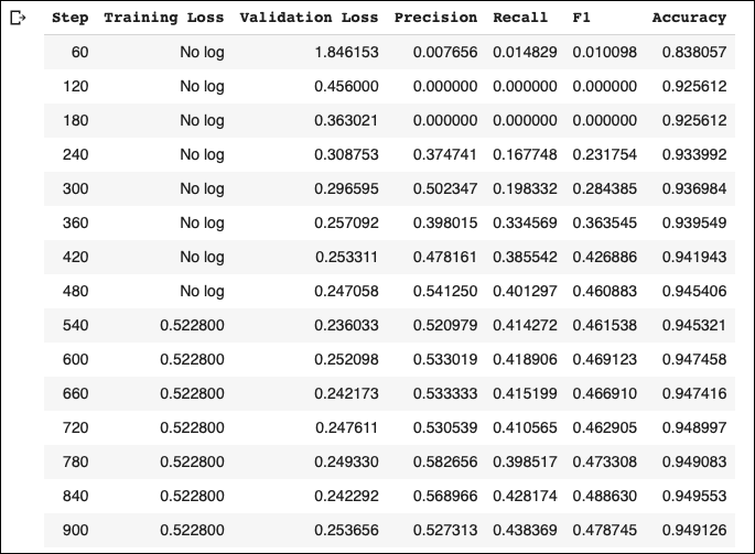
The model achieves much better validation accuracy compared to the baseline model. Also, we can achieve a better f1-score if we use a larger model, or let the model train for more epochs without applying the EarlyStopping callback.
We use the same methodology as before for our test set.
The seqeval metric also outputs the per-class metrics:
The location and person entities achieve the best scores, while group has the lowest score.
Finally, we create a function that performs entity recognition on our own sentences:
Let’s try a few examples:
The model has successfully tagged the two countries! Take a look at the United States:
- “United” was correctly tagged as
B-location. - “States” was correctly tagged as
I-location.
Again, Apple was correctly tagged as a corporation. Also, our model correctly identified and recognized the Apple products.
Named Entity Recognition is a fundamental NLP task that has numerous practical applications.
Even though the HugginFace library has created a super-friendly API for this process, there are still a few points of confusion.
I hope this tutorial has shed some light on them. The source code of this article can be found here
From data preparation to model training for NER tasks — and how to tag your own sentences
Nowadays, NLP has become synonymous with Deep Learning.
But, Deep Learning is not the ‘magic bullet’ for every NLP task. For example, in sentence classification tasks, a simple linear classifier could work reasonably well. Especially if you have a small training dataset.
However, some NLP tasks flourish with Deep Learning. One such task is Named Entity Recognition — NER:
NER is the process of identifying and classifying named entities into predefined entity categories.
For instance, in the sentence:
Nick lives in Greece and works a Data Scientist.
We have 2 entities:
- Nick, which is a ‘Person’.
- Greece, which is a ‘Location’.
Therefore, given the above sentence, a classifier should be able to locate the two terms (‘Nick’, ‘Greece’) and correctly classify them as ‘Person’ and ‘Location’ respectively.
In this tutorial, we will build a NER model, using HugginFace Transformers.
Let’s dive in!
We will use the wnut_17[1] dataset that is already included in the HugginFace Datasets library.
Explore the dataset
This dataset focuses on identifying unusual, previously-unseen entities in the context of emerging discussions. It contains 5690 documents, partitioned into training, validation, and test sets. The text sentences are tokenized into words. Let’s load the dataset:
wnut = load_dataset(“wnut_17”)
We get the following:
Next, we print the ner_tags — the predefined entities of our model:
Each ner_tag describes an entity. It can be one of the following: corporation, creative-work, group, location, person, and product.
The letter that prefixes each ner_tag indicates the token position of the entity:
- B– indicates the beginning of an entity.
- I– indicates a token is contained inside the same entity (e.g., the “York” token is a part of the “New York” entity).
- 0 indicates the token doesn’t correspond to any entity.
We also created the id2tag dictionary that maps each label to its ner_tag — this will come in handy later.
Reorganize train & validation datasets
Our dataset is not that large. Remember, Transformers require lots of data to take advantage of their superior performance.
To solve this issue, we concatenate training and validation datasets into a single training dataset. The test dataset will remain as-is for validation purposes:
A training example
Let’s print the 3rd training example from our dataset. We will use that example as a reference throughout this tutorial:
The ‘Pxleyes’ token is classified as B-corporation (the beginning of a corporation). The rest of the tokens are irrelevant — they do not represent any entity.
Next, we tokenize our data. Contrary to other use cases, tokenization for NER tasks requires special handling.
We will use the bert-base-uncased model and tokenizer from the HugginFace library.
Transformer models mostly use sub-word-based tokenizers.
During tokenization, some words could be split into two or more words. This is a standard practice because rare words could be decomposed into meaningful tokens. For example, BERT models implement by default the Byte-Pair Encoding (BPE) tokenization.
Let’s tokenize our sample training example to see how this works:
This is the original training example:
And this is how the training example is tokenized by BERT’s tokenizer:
Notice that there are two significant issues:
- The special tokens
[CLS]and[SEP]are added. - The token “Pxleyes” is split into 3 sub-tokens :
p,##xleyand##es.
In other words, the tokenization creates a mismatch between the inputs and the labels. Hence, we realign tokens and labels in the following way:
- Each single word token is mapped to its corresponding
ner_tag. - We assign the label
-100to the special tokens[CLS]and[SEP]so the loss function ignores them. By default, PyTorch ignores the-100value during loss calculation. - For subwords, we only label the first token of a given word. Thus, we assign
-100to other subtokens from the same word.
For example, the token Pxleyes is labeled as 1 (B-corporation). It is tokenized as [‘p’, ‘##xley’, ‘##es’] and after token alignment the labels should become [1, -100, -100]
We implement this functionality in the tokenize_and_align_labels() function:
And that’s it! Let’s call our custom tokenization function:
The table below shows exactly the tokenization output for our sample training example:
We are now ready to build our Deep Learning model.
We load the bert-base-uncased pretrained model and fine-tune it using our data.
But first, we should train a naive classifier to use as a baseline model.
Baseline Model
The most obvious choice for a baseline classifier is to tag every token with the most frequent entity throughout the entire training dataset— the O entity:
The baseline classifier becomes less naive if we tag each token with the most frequent label of the sentence it belongs:
Therefore, we use the second model as a baseline.
BERT for Named Entity Recognition
The Data Collator batches training examples together while applying padding to make them all the same size. The collator pads not only the inputs but also the labels:
Regarding evaluation, since our dataset is imbalanced, we can’t rely only on accuracy.
Therefore, we will also measure precision and recall. Here, we will load the seqeval metric which is included in the datasets library. This metric is commonly used for POS (Part-of-speech) tagging and NER tasks.
Let’s apply it to our reference training example and see how this works:
Note: Remember, the loss function ignores all tokens tagged with -100 during training. Our evaluation function should also take into account this information.
Hence, the compute_metrics function is defined a bit differently — we calculate precision, recall, f1-score, and accuracy by ignoring everything tagged with -100:
Finally, we instantiate the Trainer class to fine-tune our model. Notice the usage of the EarlyStopping callback:
These are our training metrics:
The model achieves much better validation accuracy compared to the baseline model. Also, we can achieve a better f1-score if we use a larger model, or let the model train for more epochs without applying the EarlyStopping callback.
We use the same methodology as before for our test set.
The seqeval metric also outputs the per-class metrics:
The location and person entities achieve the best scores, while group has the lowest score.
Finally, we create a function that performs entity recognition on our own sentences:
Let’s try a few examples:
The model has successfully tagged the two countries! Take a look at the United States:
- “United” was correctly tagged as
B-location. - “States” was correctly tagged as
I-location.
Again, Apple was correctly tagged as a corporation. Also, our model correctly identified and recognized the Apple products.
Named Entity Recognition is a fundamental NLP task that has numerous practical applications.
Even though the HugginFace library has created a super-friendly API for this process, there are still a few points of confusion.
I hope this tutorial has shed some light on them. The source code of this article can be found here
Denial of responsibility! Techno Blender is an automatic aggregator of the all world’s media. In each content, the hyperlink to the primary source is specified. All trademarks belong to their rightful owners, all materials to their authors. If you are the owner of the content and do not want us to publish your materials, please contact us by email – [email protected]. The content will be deleted within 24 hours.