
Newton’s Laws of Motion: The Original Gradient Descent
Exploring the shared language of gradient descent and Newton's motion equations
I remember the first course on Machine Learning I took during undergrad as a physics student in the school of engineering. In other words, I was an outsider. While the professor explained the backpropagation algorithm via gradient descent, I had this somewhat vague question in my head: "Is gradient descent a random algorithm?" Before raising my hand to ask the professor, the non-familiar environment made me think twice; I shrunk a little bit. Suddenly, the answer struck me.
Here's what I thought.
Gradient Descent
To say what gradient descent is, first we need to define the problem of training a neural network, and we can do this with an overview of how machines learn.
Overview of a neural network training
In all supervised neural network tasks, we have a prediction and the true value. The larger the difference between the prediction and the true value, the worse our neural network is when it comes to predicting the values. Hence, we create a function called the loss function, usually denoted as L, that quantifies how much difference there is between the actual value and the predicted value. The task of training the neural network is to update the weights and biases (for short, the parameters) to minimize the loss function. That's the big picture of training a neural network, and "learning" is simply updating the parameters to fit actual data best, i.e., minimizing the loss function.
Optimizing via gradient descent
Gradient descent is one of the optimization techniques used to calculate these new parameters. Since our task is to choose the parameters to minimize the loss function, we need a criterion for such a choice. The loss function that we are trying to minimize is a function of the neural network output, so mathematically we express it as L = L(y_nn, y). But the neural network output y_nn also depends on its parameters, so y_nn = y_nn(θ), where θ is a vector containing all the parameters of our neural network. In other words, the loss function itself is a function of the neural networks' parameters.
Borrowing some concepts from vector calculus, we know that to minimize a function, you need to go against its gradient, since the gradient points in the direction of the fastest increase of the function. To gain some intuition, let's take a look at what L(θ) might look like in Fig. 1.
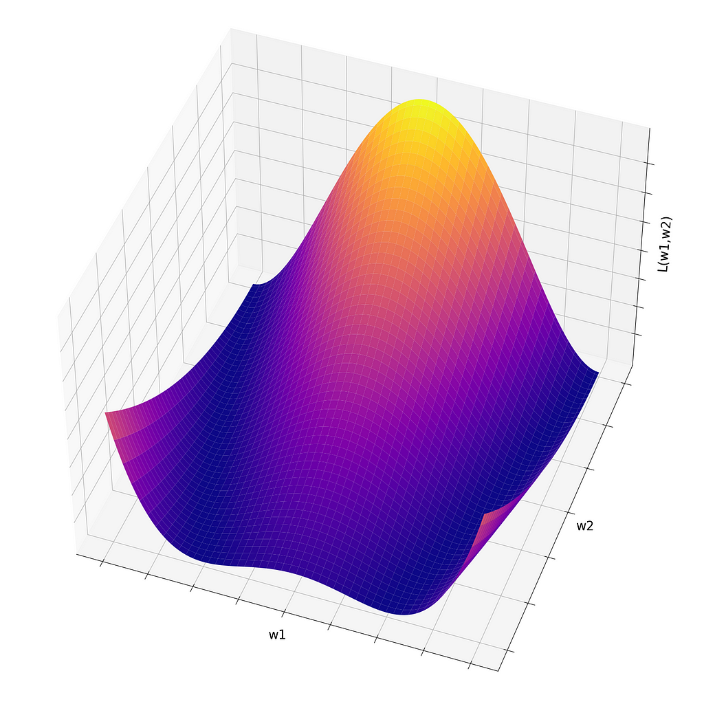
Here, we have a clear intuition of what is desirable and what is not when training a neural network: we want the values of the loss function to be smaller, so if we start with parameters w1 and w2 that result in a loss function in the yellow/orange region, we want to slide down to the surface in the direction of the purple region.
This "sliding down" motion is achieved through the gradient descent method. If we are placed at the brightest region on the surface, the gradient will continue to point up, since it's the direction of maximally fast increase. Then, going in the opposite direction (hence, gradient descent) creates a motion onto the region of maximally fast decrease.
To see this, we can plot the gradient descent vector, as displayed in Fig. 2. In this figure, we have a contour plot that shows the same region and the same function displayed in Fig. 1, but the values of the loss function are now encoded into the color: the brighter, the larger.

We can see that if we pick a point in the yellow/orange region, the gradient descent vector points in the direction that arrives the fastest in the purple region.
A nice disclaimer is that usually a neural network may contain an arbitrarily large number of parameters (GPT 3 has over 100 billion parameters!), which means that these nice visualizations are completely unpractical in real-life applications, and parameter optimization in neural networks is usually a very high-dimensional problem.
Mathematically, the gradient descent algorithm is then given by

Here, θ_(n+1) are the updated parameters (the result of sliding down the surface of Fig. 1); θ_(n) are the parameters that we started with; ρ is called the learning rate (how big is the step towards the direction where the gradient descent is pointing); and ∇L is the gradient of the loss function calculated at the initial point θ_(n). What gives the name descent here is the minus sign in front of it.
Mathematics is key here because we'll see that Newton's Second Law of Motion has the same mathematical formulation as the gradient descent equation.
Newton's Second Law
Newton's second law of motion is probably one of the most important concepts in classical mechanics since it tells how force, mass, and acceleration are tied together. Everybody knows the high school formulation of Newton's second law:

where F is the force, m is the mass, and a the acceleration. However, Newton's original formulation was in terms of a deeper quantity: momentum. Momentum is the product between the mass and the velocity of a body:

and can be interpreted as the quantity of movement of a body. The idea behind Newton's second law is that to change the momentum of a body, you need to disturb it somehow, and this disturbance is called a force. Hence, a neat formulation of Newton's second law is

This formulation works for every force you can think of, but we would like a little more structure in our discussion and, to gain structure, we need to constrain our domain of possibilities. Let's talk about conservative forces and potentials.
Conservative forces and potentials
A conservative force is a force that does not dissipate energy. It means that, when we are in a system with only conservative forces involved, the total energy is a constant. This must sound very restrictive, but in reality, the most fundamental forces in nature are conservative, such as gravity and electric force.
For each conservative force, we associate something called a potential. This potential is related to the force via the equation

in one dimension. If we take a closer look at the last two equations presented, we arrive at the second law of motion for conservative fields:

Since derivatives are kind of complicated to deal with, and in computer sciences we approximate derivatives as finite differences anyway, let's replace d's with Δ's:

We know that Δ means "take the updated value and subtract by the current value". Hence, we can re-write the formula above as

This already looks pretty similar to the gradient descent equation shown in some lines above. To make it even more similar, we just have to look at it in three dimensions, where the gradient arises naturally:

We see a clear correspondence between the gradient descent and the formulation shown above, which completely derives from Newtonian physics. The momentum of a body (and you can read this as velocity if you prefer) will always point toward the direction where the potential decreases the fastest, with a step size given by Δt.
Final words and takeaways
So we can relate the potential, within the Newtonian formulation, to the loss function in machine learning. The momentum vector is similar to the parameter vector, which we are trying to optimize, and the time step constant is the learning rate, i.e., how fast we are moving towards the minimum of the loss function. Hence, the similar mathematical formulation shows that these concepts are tied together and present a nice, unified way of looking at them.
If you are wondering, the answer to my question at the beginning is "no". There is no randomness in the gradient descent algorithm since it replicates what nature does every day: the physical trajectory of a particle always tries to find a way to rest in the lowest possible potential around it. If you let a ball fall from a certain hight, it will always have the same trajectory, no randomness. When you see someone on a skateboard sliding down a steep ramp, remember: that's literally nature applying the gradient descent algorithm.
The way we see a problem may influence its solution. In this article, I have not shown you anything new in terms of computer science or physics (indeed, the physics presented here is ~400 years old), but shifting the perspective and tying (apparently) non-related concepts together may create new links and intuitions about a topic.
References
[1] Robert Kwiatkowski, Gradient Descent Algorithm — a deep dive, 2021.
[2] Nivaldo A. Lemos, Analytical Mechanics, Cambridge University Press, 2018.
Newton’s Laws of Motion: The Original Gradient Descent was originally published in Towards Data Science on Medium, where people are continuing the conversation by highlighting and responding to this story.
Exploring the shared language of gradient descent and Newton's motion equations

I remember the first course on Machine Learning I took during undergrad as a physics student in the school of engineering. In other words, I was an outsider. While the professor explained the backpropagation algorithm via gradient descent, I had this somewhat vague question in my head: "Is gradient descent a random algorithm?" Before raising my hand to ask the professor, the non-familiar environment made me think twice; I shrunk a little bit. Suddenly, the answer struck me.
Here's what I thought.
Gradient Descent
To say what gradient descent is, first we need to define the problem of training a neural network, and we can do this with an overview of how machines learn.
Overview of a neural network training
In all supervised neural network tasks, we have a prediction and the true value. The larger the difference between the prediction and the true value, the worse our neural network is when it comes to predicting the values. Hence, we create a function called the loss function, usually denoted as L, that quantifies how much difference there is between the actual value and the predicted value. The task of training the neural network is to update the weights and biases (for short, the parameters) to minimize the loss function. That's the big picture of training a neural network, and "learning" is simply updating the parameters to fit actual data best, i.e., minimizing the loss function.
Optimizing via gradient descent
Gradient descent is one of the optimization techniques used to calculate these new parameters. Since our task is to choose the parameters to minimize the loss function, we need a criterion for such a choice. The loss function that we are trying to minimize is a function of the neural network output, so mathematically we express it as L = L(y_nn, y). But the neural network output y_nn also depends on its parameters, so y_nn = y_nn(θ), where θ is a vector containing all the parameters of our neural network. In other words, the loss function itself is a function of the neural networks' parameters.
Borrowing some concepts from vector calculus, we know that to minimize a function, you need to go against its gradient, since the gradient points in the direction of the fastest increase of the function. To gain some intuition, let's take a look at what L(θ) might look like in Fig. 1.
Here, we have a clear intuition of what is desirable and what is not when training a neural network: we want the values of the loss function to be smaller, so if we start with parameters w1 and w2 that result in a loss function in the yellow/orange region, we want to slide down to the surface in the direction of the purple region.
This "sliding down" motion is achieved through the gradient descent method. If we are placed at the brightest region on the surface, the gradient will continue to point up, since it's the direction of maximally fast increase. Then, going in the opposite direction (hence, gradient descent) creates a motion onto the region of maximally fast decrease.
To see this, we can plot the gradient descent vector, as displayed in Fig. 2. In this figure, we have a contour plot that shows the same region and the same function displayed in Fig. 1, but the values of the loss function are now encoded into the color: the brighter, the larger.
We can see that if we pick a point in the yellow/orange region, the gradient descent vector points in the direction that arrives the fastest in the purple region.
A nice disclaimer is that usually a neural network may contain an arbitrarily large number of parameters (GPT 3 has over 100 billion parameters!), which means that these nice visualizations are completely unpractical in real-life applications, and parameter optimization in neural networks is usually a very high-dimensional problem.
Mathematically, the gradient descent algorithm is then given by
Here, θ_(n+1) are the updated parameters (the result of sliding down the surface of Fig. 1); θ_(n) are the parameters that we started with; ρ is called the learning rate (how big is the step towards the direction where the gradient descent is pointing); and ∇L is the gradient of the loss function calculated at the initial point θ_(n). What gives the name descent here is the minus sign in front of it.
Mathematics is key here because we'll see that Newton's Second Law of Motion has the same mathematical formulation as the gradient descent equation.
Newton's Second Law
Newton's second law of motion is probably one of the most important concepts in classical mechanics since it tells how force, mass, and acceleration are tied together. Everybody knows the high school formulation of Newton's second law:
where F is the force, m is the mass, and a the acceleration. However, Newton's original formulation was in terms of a deeper quantity: momentum. Momentum is the product between the mass and the velocity of a body:
and can be interpreted as the quantity of movement of a body. The idea behind Newton's second law is that to change the momentum of a body, you need to disturb it somehow, and this disturbance is called a force. Hence, a neat formulation of Newton's second law is
This formulation works for every force you can think of, but we would like a little more structure in our discussion and, to gain structure, we need to constrain our domain of possibilities. Let's talk about conservative forces and potentials.
Conservative forces and potentials
A conservative force is a force that does not dissipate energy. It means that, when we are in a system with only conservative forces involved, the total energy is a constant. This must sound very restrictive, but in reality, the most fundamental forces in nature are conservative, such as gravity and electric force.
For each conservative force, we associate something called a potential. This potential is related to the force via the equation
in one dimension. If we take a closer look at the last two equations presented, we arrive at the second law of motion for conservative fields:
Since derivatives are kind of complicated to deal with, and in computer sciences we approximate derivatives as finite differences anyway, let's replace d's with Δ's:
We know that Δ means "take the updated value and subtract by the current value". Hence, we can re-write the formula above as
This already looks pretty similar to the gradient descent equation shown in some lines above. To make it even more similar, we just have to look at it in three dimensions, where the gradient arises naturally:
We see a clear correspondence between the gradient descent and the formulation shown above, which completely derives from Newtonian physics. The momentum of a body (and you can read this as velocity if you prefer) will always point toward the direction where the potential decreases the fastest, with a step size given by Δt.
Final words and takeaways
So we can relate the potential, within the Newtonian formulation, to the loss function in machine learning. The momentum vector is similar to the parameter vector, which we are trying to optimize, and the time step constant is the learning rate, i.e., how fast we are moving towards the minimum of the loss function. Hence, the similar mathematical formulation shows that these concepts are tied together and present a nice, unified way of looking at them.
If you are wondering, the answer to my question at the beginning is "no". There is no randomness in the gradient descent algorithm since it replicates what nature does every day: the physical trajectory of a particle always tries to find a way to rest in the lowest possible potential around it. If you let a ball fall from a certain hight, it will always have the same trajectory, no randomness. When you see someone on a skateboard sliding down a steep ramp, remember: that's literally nature applying the gradient descent algorithm.
The way we see a problem may influence its solution. In this article, I have not shown you anything new in terms of computer science or physics (indeed, the physics presented here is ~400 years old), but shifting the perspective and tying (apparently) non-related concepts together may create new links and intuitions about a topic.
References
[1] Robert Kwiatkowski, Gradient Descent Algorithm — a deep dive, 2021.
[2] Nivaldo A. Lemos, Analytical Mechanics, Cambridge University Press, 2018.
Newton’s Laws of Motion: The Original Gradient Descent was originally published in Towards Data Science on Medium, where people are continuing the conversation by highlighting and responding to this story.
Denial of responsibility! Techno Blender is an automatic aggregator of the all world’s media. In each content, the hyperlink to the primary source is specified. All trademarks belong to their rightful owners, all materials to their authors. If you are the owner of the content and do not want us to publish your materials, please contact us by email – [email protected]. The content will be deleted within 24 hours.