
Normalize any Continuously Distributed Data with a Couple of Lines of Code | by Danil Vityazev | Sep, 2022
How to use inverse transform sampling to improve your model
Normalizing data is a common task in data science. Sometimes it allows us to speed up gradient descent or improve model accuracy, and in some cases it absolutely crucial. For example, the model I described in my last article cannot handle targets that are distributed non-normally. Some normalization techniques, like taking a logarithm, may work most of the time, but in this case, I decided to try something that would work for any data, no matter how it was initially distributed. The method I’ll describe below is based on inverse transform sampling: the main idea is to construct such function F, based on the data’s statistical properties, so F(x) is distributed normally. Here’s how to do it.
The algorithm I’m talking about is based on the inverse transform sampling method. This method is widely used in pseudo-random number generators to generate numbers from any given distribution. Having uniformly distributed data you can always transform it into distribution, with any given cumulative density function (or CDF for short). A CDF shows what proportion of data points of distribution is smaller than a given value and basically denotes all the statistical properties of the distribution.
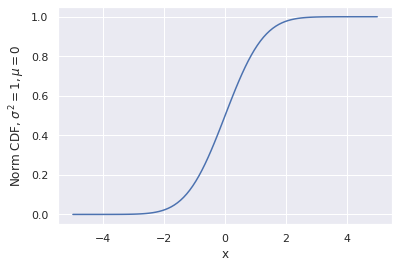
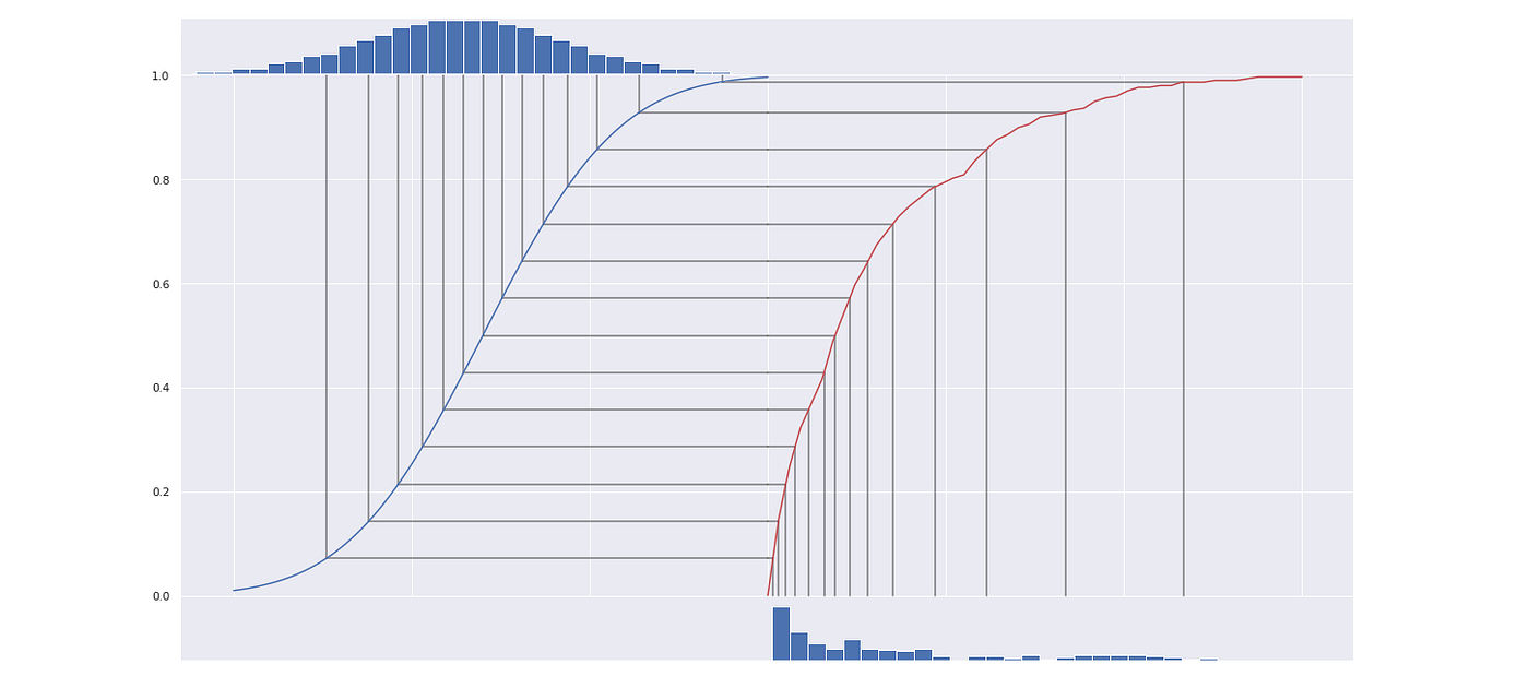
The main idea is that for any continuously distributed data xᵢ, CDF(xᵢ) is distributed uniformly. In other words, to get uniformly distributed data one just takes a CDF of each point. The mathematical proof of this statement is out of the scope of this article, but the fact that said operation is essentially just sorting all the values and replacing each value with its number gives it an intuitive sense.

In the gif above you can see how it works. I generated some messy distributed data and then calculated its CDF (the red line) and transformed the date with it. Now the data is uniformly distributed.
Calculating CDF is easier than it seems. Remember, a CDF is a fraction of data smaller than the given one.
def CDF(x, data):
return sum(data <= x) / len(data)
It’s worth mentioning that a CDF in general is a bijective function, which means that the transformation is reversible. We can use this fact to transform obtained uniform distribution into any distribution we want, say normal distribution. In order to do that we need to compute an inverse CDF of the distribution we want to get. Generally, it’s not the easiest task. The function we need is called a percent point function, or PPF for short. Luckily for us, the PPFs of any major distribution are accessible through the SciPy library, and one doesn’t need to compute it themselves.
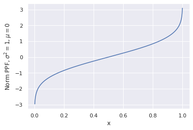
Here’s how to interpret it: for any argument x between 0 and 1 PPF returns the maximum value for the point to fit into x’th percentile. At the same time being the inverse function of a CDF it looks like a function from the first picture, just rotated 90°.
Now we have a nice normal distribution as desired. Finally, to make a function that transforms our initial data, all we have to do to merge these two operations together into one function:
from scipy.stats import normdef normalize(x, data):
x_uniform = CDF(x, data)
return norm.ppf(x_uniform)
The red line in the picture above represents the final transform function.
By the way, we can easily transform data into any other distribution just by replacing PPF with one of the desired distribution. Here is the transformation of our messy data into lognormal distribution. Notice how the transforming curve is different.
Notice how the final transformation is always monotonic. That means that no two points are swapped after the transformation. If the value of the initial feature is greater for one point than for another, after the transformation, the transformed value will also be greater for that point. This fact allows this algorithm to be applied to data science tasks.
To sum up, unlike more common methods, the algorithm described in this article doesn’t require any assumptions about initial distribution. At the same time, the output data follows the normal distribution extremely precisely. This method has been shown to increase the accuracy of models, that assume input data distribution. For example, the Bayesian model from the last article has R² ~ 0.2 without data normalization and R² of 0.34 with normalized data. Linear models have also shown improvements in R² on 3–5 percentage points on normalized data.
That’s it. Thanks for your time, and I hope you found this article useful!
How to use inverse transform sampling to improve your model
Normalizing data is a common task in data science. Sometimes it allows us to speed up gradient descent or improve model accuracy, and in some cases it absolutely crucial. For example, the model I described in my last article cannot handle targets that are distributed non-normally. Some normalization techniques, like taking a logarithm, may work most of the time, but in this case, I decided to try something that would work for any data, no matter how it was initially distributed. The method I’ll describe below is based on inverse transform sampling: the main idea is to construct such function F, based on the data’s statistical properties, so F(x) is distributed normally. Here’s how to do it.
The algorithm I’m talking about is based on the inverse transform sampling method. This method is widely used in pseudo-random number generators to generate numbers from any given distribution. Having uniformly distributed data you can always transform it into distribution, with any given cumulative density function (or CDF for short). A CDF shows what proportion of data points of distribution is smaller than a given value and basically denotes all the statistical properties of the distribution.
The main idea is that for any continuously distributed data xᵢ, CDF(xᵢ) is distributed uniformly. In other words, to get uniformly distributed data one just takes a CDF of each point. The mathematical proof of this statement is out of the scope of this article, but the fact that said operation is essentially just sorting all the values and replacing each value with its number gives it an intuitive sense.
In the gif above you can see how it works. I generated some messy distributed data and then calculated its CDF (the red line) and transformed the date with it. Now the data is uniformly distributed.
Calculating CDF is easier than it seems. Remember, a CDF is a fraction of data smaller than the given one.
def CDF(x, data):
return sum(data <= x) / len(data)
It’s worth mentioning that a CDF in general is a bijective function, which means that the transformation is reversible. We can use this fact to transform obtained uniform distribution into any distribution we want, say normal distribution. In order to do that we need to compute an inverse CDF of the distribution we want to get. Generally, it’s not the easiest task. The function we need is called a percent point function, or PPF for short. Luckily for us, the PPFs of any major distribution are accessible through the SciPy library, and one doesn’t need to compute it themselves.
Here’s how to interpret it: for any argument x between 0 and 1 PPF returns the maximum value for the point to fit into x’th percentile. At the same time being the inverse function of a CDF it looks like a function from the first picture, just rotated 90°.
Now we have a nice normal distribution as desired. Finally, to make a function that transforms our initial data, all we have to do to merge these two operations together into one function:
from scipy.stats import normdef normalize(x, data):
x_uniform = CDF(x, data)
return norm.ppf(x_uniform)
The red line in the picture above represents the final transform function.
By the way, we can easily transform data into any other distribution just by replacing PPF with one of the desired distribution. Here is the transformation of our messy data into lognormal distribution. Notice how the transforming curve is different.
Notice how the final transformation is always monotonic. That means that no two points are swapped after the transformation. If the value of the initial feature is greater for one point than for another, after the transformation, the transformed value will also be greater for that point. This fact allows this algorithm to be applied to data science tasks.
To sum up, unlike more common methods, the algorithm described in this article doesn’t require any assumptions about initial distribution. At the same time, the output data follows the normal distribution extremely precisely. This method has been shown to increase the accuracy of models, that assume input data distribution. For example, the Bayesian model from the last article has R² ~ 0.2 without data normalization and R² of 0.34 with normalized data. Linear models have also shown improvements in R² on 3–5 percentage points on normalized data.
That’s it. Thanks for your time, and I hope you found this article useful!
Denial of responsibility! Techno Blender is an automatic aggregator of the all world’s media. In each content, the hyperlink to the primary source is specified. All trademarks belong to their rightful owners, all materials to their authors. If you are the owner of the content and do not want us to publish your materials, please contact us by email – [email protected]. The content will be deleted within 24 hours.