
Object Detection Neural Network: Building a YOLOX Model on a Custom Dataset | by Nahid Alam | Jun, 2022
A Comprehensive Guide
In Computer Vision — object detection is the task of detecting an object in an image or video. The job of an object detection algorithm is two fold
- a localization task — outputs the bounding box (x, y coordinate). In essence, the localization task is a regression problem that outputs continuous numbers representing the bounding box coordinates.
- a classification task — classifies an object (person vs car etc.).
Object detection algorithms can be based on traditional Computer Vision approaches or Neural Network ones [1]. Among the Neural Network based approaches — we can classify the algorithms in two main categories — single stage and two stage object detector.
In a single-stage object detector — the task of localization and classification is done in one pass — meaning there is no additional network to “help” the localization and classification process of the object detector. Single-stage detectors yields higher inference speed and preferable for mobile and edge devices. The YOLO family of object detection algorithms are single-stage object detector.
In a two-stage detector — in addition to the localization and classification network, we have an additional network called Region Proposal Network (RPN). RPN is used to decide “where” to look in order to reduce the computational requirements of the overall object detection network. RPN uses anchors — fixed sized reference bounding boxes which are placed uniformly throughout the original image. In the region proposal stage [2] — we ask
- Does this anchor contain a relevant object?
- How do we adjust the anchor to better fit the relevant object?
Once we have a list from the above process, the task of localization and classification network becomes straight-forward. Two-stage detectors have generally higher localization and classification accuracy. RCNN, Faster-RCNN etc. are a few examples of two stage object detectors.
An image is an input to an object detection network. The input is passed through a Convolutional Neural Network (CNN) backbone to extract features (embedding) out of it. The job of the neck stage is to mix and combine the features formed in the CNN backbone to prepare for the head step. The components of the neck typically flow up and down among layers and connect only the few layers at the end of the [7]. The head is responsible for the prediction — aka. classification and localization.

YOLO family of object detectors [3] are the state-of-the-art (SOTA) single stage object detectors. YOLO family has evolved from YOLOv1 since its inception in 2016 to this date with YOLOX in 2021. In this article, our focus will be on YOLOX.

Lets look at a few architectural components of YOLOX.
Decoupled Head
With YOLOv3-v5, the detection head remained coupled. This posed a challenge as the detection head is basically doing two different tasks — classification and regression (bounding box). Replacing YOLO’s head with a decoupled one — one for classification and the other for bounding box regression.
Strong Data Augmentation
YOLOX added two data augmentation strategies — Mosaic and MixUp.
- Mosaic was originally introduced in YOLOv3 and subsequently used in v4 and v5. Mosaic data augmentation combines 4 training images into one in certain ratios. This allows for the model to learn how to identify objects at a smaller scale than normal. It also is useful in training to significantly reduce the need for a large mini-batch size [4].
- MixUp — is a data augmentation technique that that generates a weighted combinations of random image pairs from the training data [5].
Anchor-free Architecture
YOLOv3-5 were anchor based pipeline — meaning the RPN style fixed sized reference bounding boxes which are placed uniformly throughout the original image to check if this box contains an expected class. Anchor boxes allow us to find more than one object in the same grid. But anchor based mechanisms has some problems too —
- In anchor-based mechanism, optimal anchor boxes should be determined for object detection. To do that, we need to find optimal anchor boxes with clustering analysis before training. This is an extra step that increase training time and complexity.
- Another problem is that the anchor-based mechanism increases the number of predictions to be made for each image. This will increase the inference time.
- And finally, anchor-based mechanism significantly increases the complexity of the detection head and the overall network.
In recent years, anchor-free mechanisms were improved but were not brought into the YOLO family until YOLOX.
Anchor-free YOLOX reduces number of prediction for each image cell from 3 to 1.
SimOTA
SimOTA is an advanced label assignment technique. What is label assignment? It defines positive/negative training samples for each ground truth object. YOLOX formulates this label assignment problem as an Optimal Transport (OT) problem [6].
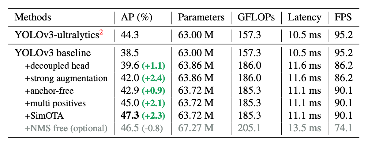
Below table shows how these different architecture components help improve the Average Precision (AP) of the model over baseline.
Installation
You can find the open source code for YOLOX here. Following the installation section, you can install from the source
git clone [email protected]:Megvii-BaseDetection/YOLOX.git
cd YOLOX
pip3 install -v -e .  # or  python3 setup.py develop
Dataset Conversion
Make sure your custom dataset is in COCO format. If your dataset is in darknet or yolo5 format, you can use YOLO2COCO repository to convert it to COCO format.
Download Pre-trained Weight
When training our model on custom dataset, we prefer to start with a pretrained baseline and train on our data on top of it.
wget https://github.com/Megvii-BaseDetection/storage/releases/download/0.0.1/yolox_s.pth
Model Training
A critical component of YOLOX model training is to have the right experiment file — a few sample custom experiment files are here.
#!/usr/bin/env python3
# -*- coding:utf-8 -*-
# Copyright (c) Megvii, Inc. and its affiliates.
import osfrom yolox.exp import Exp as MyExp
class Exp(MyExp):
def __init__(self):
super(Exp, self).__init__()
self.depth = 0.33
self.width = 0.50
self.exp_name = os.path.split(os.path.realpath(__file__))[1].split(".")[0]
# Define yourself dataset path
self.data_dir = "datasets/coco128"
self.train_ann = "instances_train2017.json"
self.val_ann = "instances_val2017.json"
self.num_classes = 71
self.max_epoch = 300
self.data_num_workers = 4
self.eval_interval = 1
You can experiment with the variables such as self.num_classes based on the number of classes you have, change dataset path etc.
You can see another example of a custom experiment file here
import os
from yolox.exp import Exp as MyExpclass Exp(MyExp):
def __init__(self):
super(Exp, self).__init__()
self.depth = 0.33
self.width = 0.50
self.exp_name = os.path.split(os.path.realpath(__file__))[1].split(".")[0]
# Define yourself dataset path
self.data_dir = "data"
self.train_ann = "train.json"
self.val_ann = "val.json"
self.num_classes = 1
self.data_num_workers = 4
self.eval_interval = 1
# --------------- transform config ----------------- #
self.degrees = 10.0
self.translate = 0.1
self.scale = (0.1, 2)
self.mosaic_scale = (0.8, 1.6)
self.shear = 2.0
self.perspective = 0.0
self.enable_mixup = True
# -------------- training config --------------------- #
self.warmup_epochs = 5
self.max_epoch = 300
self.warmup_lr = 0
self.basic_lr_per_img = 0.01 / 64.0
self.scheduler = "yoloxwarmcos"
self.no_aug_epochs = 15
self.min_lr_ratio = 0.05
self.ema = True
self.weight_decay = 5e-4
self.momentum = 0.9
To train the model (make sure you are in the YOLOX directory), you can use below command. Note the parameters of d and b. d indicates the number of GPU, in my case it is 1. b is the batch size during training which is 8x the value of d.
python tools/train.py -f exps/example/custom/yolox_tiny.py -d 1 -b 8 --fp16 -o -c yolox_tiny.pth
Model Evaluation
During model evaluation, you have to specify the same (or a copy of it) experiment file that you used for training
python -m yolox.tools.eval -n yolox_s -c YOLOX_outputs/yolox_s/best_ckpt.pth -f exps/example/custom/yolox_s.py -b 1 -d 1 --conf 0.001 --fp16 --fuse
Model Testing
To run YOLOX inference on test image, we can do below [8]
TEST_IMAGE_PATH = "test_image.jpg"python tools/demo.py image -f exps/example/custom/yolox_s.py -c YOLOX_outputs/yolox_s/best_ckpt.pth --path {TEST_IMAGE_PATH} --conf 0.25 --nms 0.45 --tsize 640 --save_result --device gpu
Let’s say the output prediction image is prediction.jpg. You can visualize this image like below
from PIL import Image
Image.open('prediction.jpg')
To check how your model performs on a video, you can do below
python tools/demo.py video -n yolox-s -c /path/to/your/yolox_s.pth -f exps/example/custom/yolox_s.py --path /path/to/your/video --conf 0.25 --nms 0.45 --tsize 640 --save_result --device [cpu/gpu]
Note the parameter conf here — it indicates the confidence interval, meaning how confident you want your model to be before it outputs a bounding box. Having a higher conf score generally increases the quality of your detection — removing unwanted bounding box etc.
Path Forward:
Now that we learned how to train YOLOX on a custom dataset — there are many possibilities ahead. Depending on your use-case, you might want a lighter or heavier version of YOLOX. You can experiment with the parameters in the experiment file defined in `exps/example/custom/yolox_s.py. Once the model is ready, depending on your usecase you might need to prune or quantize the model — specifically if you are deploying it on an edge device.
I hope you enjoyed this blog post. Feel free to comment here if you have any question.
References:
- Object Detection in 20 Years: A Survey https://arxiv.org/pdf/1905.05055.pdf
- One-stage vs two-stage object detector https://stackoverflow.com/questions/65942471/one-stage-vs-two-stage-object-detection
- Introduction to the YOLO family https://pyimagesearch.com/2022/04/04/introduction-to-the-yolo-family/
- YOLOv4 data augmentation https://blog.roboflow.com/yolov4-data-augmentation/
- MixUp https://paperswithcode.com/method/mixup
- Optimal Transport Assignment for Object Detection https://arxiv.org/pdf/2103.14259.pdf
- A thorough breakdown of YOLOv4 https://blog.roboflow.com/a-thorough-breakdown-of-yolov4/
- How to train a custom YOLOX model https://blog.roboflow.com/how-to-train-yolox-on-a-custom-dataset/
A Comprehensive Guide

In Computer Vision — object detection is the task of detecting an object in an image or video. The job of an object detection algorithm is two fold
- a localization task — outputs the bounding box (x, y coordinate). In essence, the localization task is a regression problem that outputs continuous numbers representing the bounding box coordinates.
- a classification task — classifies an object (person vs car etc.).
Object detection algorithms can be based on traditional Computer Vision approaches or Neural Network ones [1]. Among the Neural Network based approaches — we can classify the algorithms in two main categories — single stage and two stage object detector.
In a single-stage object detector — the task of localization and classification is done in one pass — meaning there is no additional network to “help” the localization and classification process of the object detector. Single-stage detectors yields higher inference speed and preferable for mobile and edge devices. The YOLO family of object detection algorithms are single-stage object detector.
In a two-stage detector — in addition to the localization and classification network, we have an additional network called Region Proposal Network (RPN). RPN is used to decide “where” to look in order to reduce the computational requirements of the overall object detection network. RPN uses anchors — fixed sized reference bounding boxes which are placed uniformly throughout the original image. In the region proposal stage [2] — we ask
- Does this anchor contain a relevant object?
- How do we adjust the anchor to better fit the relevant object?
Once we have a list from the above process, the task of localization and classification network becomes straight-forward. Two-stage detectors have generally higher localization and classification accuracy. RCNN, Faster-RCNN etc. are a few examples of two stage object detectors.
An image is an input to an object detection network. The input is passed through a Convolutional Neural Network (CNN) backbone to extract features (embedding) out of it. The job of the neck stage is to mix and combine the features formed in the CNN backbone to prepare for the head step. The components of the neck typically flow up and down among layers and connect only the few layers at the end of the [7]. The head is responsible for the prediction — aka. classification and localization.
YOLO family of object detectors [3] are the state-of-the-art (SOTA) single stage object detectors. YOLO family has evolved from YOLOv1 since its inception in 2016 to this date with YOLOX in 2021. In this article, our focus will be on YOLOX.
Lets look at a few architectural components of YOLOX.
Decoupled Head
With YOLOv3-v5, the detection head remained coupled. This posed a challenge as the detection head is basically doing two different tasks — classification and regression (bounding box). Replacing YOLO’s head with a decoupled one — one for classification and the other for bounding box regression.
Strong Data Augmentation
YOLOX added two data augmentation strategies — Mosaic and MixUp.
- Mosaic was originally introduced in YOLOv3 and subsequently used in v4 and v5. Mosaic data augmentation combines 4 training images into one in certain ratios. This allows for the model to learn how to identify objects at a smaller scale than normal. It also is useful in training to significantly reduce the need for a large mini-batch size [4].
- MixUp — is a data augmentation technique that that generates a weighted combinations of random image pairs from the training data [5].
Anchor-free Architecture
YOLOv3-5 were anchor based pipeline — meaning the RPN style fixed sized reference bounding boxes which are placed uniformly throughout the original image to check if this box contains an expected class. Anchor boxes allow us to find more than one object in the same grid. But anchor based mechanisms has some problems too —
- In anchor-based mechanism, optimal anchor boxes should be determined for object detection. To do that, we need to find optimal anchor boxes with clustering analysis before training. This is an extra step that increase training time and complexity.
- Another problem is that the anchor-based mechanism increases the number of predictions to be made for each image. This will increase the inference time.
- And finally, anchor-based mechanism significantly increases the complexity of the detection head and the overall network.
In recent years, anchor-free mechanisms were improved but were not brought into the YOLO family until YOLOX.
Anchor-free YOLOX reduces number of prediction for each image cell from 3 to 1.
SimOTA
SimOTA is an advanced label assignment technique. What is label assignment? It defines positive/negative training samples for each ground truth object. YOLOX formulates this label assignment problem as an Optimal Transport (OT) problem [6].
Below table shows how these different architecture components help improve the Average Precision (AP) of the model over baseline.
Installation
You can find the open source code for YOLOX here. Following the installation section, you can install from the source
git clone [email protected]:Megvii-BaseDetection/YOLOX.git
cd YOLOX
pip3 install -v -e .  # or  python3 setup.py develop
Dataset Conversion
Make sure your custom dataset is in COCO format. If your dataset is in darknet or yolo5 format, you can use YOLO2COCO repository to convert it to COCO format.
Download Pre-trained Weight
When training our model on custom dataset, we prefer to start with a pretrained baseline and train on our data on top of it.
wget https://github.com/Megvii-BaseDetection/storage/releases/download/0.0.1/yolox_s.pth
Model Training
A critical component of YOLOX model training is to have the right experiment file — a few sample custom experiment files are here.
#!/usr/bin/env python3
# -*- coding:utf-8 -*-
# Copyright (c) Megvii, Inc. and its affiliates.
import osfrom yolox.exp import Exp as MyExp
class Exp(MyExp):
def __init__(self):
super(Exp, self).__init__()
self.depth = 0.33
self.width = 0.50
self.exp_name = os.path.split(os.path.realpath(__file__))[1].split(".")[0]
# Define yourself dataset path
self.data_dir = "datasets/coco128"
self.train_ann = "instances_train2017.json"
self.val_ann = "instances_val2017.json"
self.num_classes = 71
self.max_epoch = 300
self.data_num_workers = 4
self.eval_interval = 1
You can experiment with the variables such as self.num_classes based on the number of classes you have, change dataset path etc.
You can see another example of a custom experiment file here
import os
from yolox.exp import Exp as MyExpclass Exp(MyExp):
def __init__(self):
super(Exp, self).__init__()
self.depth = 0.33
self.width = 0.50
self.exp_name = os.path.split(os.path.realpath(__file__))[1].split(".")[0]
# Define yourself dataset path
self.data_dir = "data"
self.train_ann = "train.json"
self.val_ann = "val.json"
self.num_classes = 1
self.data_num_workers = 4
self.eval_interval = 1
# --------------- transform config ----------------- #
self.degrees = 10.0
self.translate = 0.1
self.scale = (0.1, 2)
self.mosaic_scale = (0.8, 1.6)
self.shear = 2.0
self.perspective = 0.0
self.enable_mixup = True
# -------------- training config --------------------- #
self.warmup_epochs = 5
self.max_epoch = 300
self.warmup_lr = 0
self.basic_lr_per_img = 0.01 / 64.0
self.scheduler = "yoloxwarmcos"
self.no_aug_epochs = 15
self.min_lr_ratio = 0.05
self.ema = True
self.weight_decay = 5e-4
self.momentum = 0.9
To train the model (make sure you are in the YOLOX directory), you can use below command. Note the parameters of d and b. d indicates the number of GPU, in my case it is 1. b is the batch size during training which is 8x the value of d.
python tools/train.py -f exps/example/custom/yolox_tiny.py -d 1 -b 8 --fp16 -o -c yolox_tiny.pth
Model Evaluation
During model evaluation, you have to specify the same (or a copy of it) experiment file that you used for training
python -m yolox.tools.eval -n yolox_s -c YOLOX_outputs/yolox_s/best_ckpt.pth -f exps/example/custom/yolox_s.py -b 1 -d 1 --conf 0.001 --fp16 --fuse
Model Testing
To run YOLOX inference on test image, we can do below [8]
TEST_IMAGE_PATH = "test_image.jpg"python tools/demo.py image -f exps/example/custom/yolox_s.py -c YOLOX_outputs/yolox_s/best_ckpt.pth --path {TEST_IMAGE_PATH} --conf 0.25 --nms 0.45 --tsize 640 --save_result --device gpu
Let’s say the output prediction image is prediction.jpg. You can visualize this image like below
from PIL import Image
Image.open('prediction.jpg')
To check how your model performs on a video, you can do below
python tools/demo.py video -n yolox-s -c /path/to/your/yolox_s.pth -f exps/example/custom/yolox_s.py --path /path/to/your/video --conf 0.25 --nms 0.45 --tsize 640 --save_result --device [cpu/gpu]
Note the parameter conf here — it indicates the confidence interval, meaning how confident you want your model to be before it outputs a bounding box. Having a higher conf score generally increases the quality of your detection — removing unwanted bounding box etc.
Path Forward:
Now that we learned how to train YOLOX on a custom dataset — there are many possibilities ahead. Depending on your use-case, you might want a lighter or heavier version of YOLOX. You can experiment with the parameters in the experiment file defined in `exps/example/custom/yolox_s.py. Once the model is ready, depending on your usecase you might need to prune or quantize the model — specifically if you are deploying it on an edge device.
I hope you enjoyed this blog post. Feel free to comment here if you have any question.
References:
- Object Detection in 20 Years: A Survey https://arxiv.org/pdf/1905.05055.pdf
- One-stage vs two-stage object detector https://stackoverflow.com/questions/65942471/one-stage-vs-two-stage-object-detection
- Introduction to the YOLO family https://pyimagesearch.com/2022/04/04/introduction-to-the-yolo-family/
- YOLOv4 data augmentation https://blog.roboflow.com/yolov4-data-augmentation/
- MixUp https://paperswithcode.com/method/mixup
- Optimal Transport Assignment for Object Detection https://arxiv.org/pdf/2103.14259.pdf
- A thorough breakdown of YOLOv4 https://blog.roboflow.com/a-thorough-breakdown-of-yolov4/
- How to train a custom YOLOX model https://blog.roboflow.com/how-to-train-yolox-on-a-custom-dataset/
Denial of responsibility! Techno Blender is an automatic aggregator of the all world’s media. In each content, the hyperlink to the primary source is specified. All trademarks belong to their rightful owners, all materials to their authors. If you are the owner of the content and do not want us to publish your materials, please contact us by email – [email protected]. The content will be deleted within 24 hours.