
On Data-Driven Equation Discovery
Describing the nature with the help of analytical expressions verified through experiments has been a hallmark of the success of science especially in physics from fundamental law of gravitation to quantum mechanics and beyond. As challenges such as climate change, fusion, and computational biology pivot our focus toward more compute, there is a growing need for concise yet robust reduced models that maintain physical consistency at a lower cost. Scientific machine learning is an emergent field which promises to provide such solutions. This article is a short review of recent data-driven equation discovery methods targeting scientists and engineers familiar with very basics of machine learning or statistics.
Motivation and historical perspectives
Simply fitting the data well has proven to be a short-sighted endeavour, as demonstrated by the Ptolemy’s model of geocentrism which was the most observationally accurate model until Kepler’s heliocentric one. Thus, combining observations with fundamental physical principles plays a big role in science. However, often in physics we forget the extent to which our models of the world are already data driven. Take an example of standard model of particles with 19 parameters, whose numerical values are established by experiment. Earth system models used for meteorology and climate, while running on a physically consistent core based on fluid dynamics, also require careful calibration to observations of many of their sensitive parameters. Finally, reduced order modelling is gaining traction in fusion and space weather community and will likely remain relevant in future. In fields such as biology and social sciences, where first principle approaches are less effective, statistical system identification already plays a significant role.
There are various methods in machine learning that allow predicting the evolution of the system directly from data. More recently, deep neural networks have achieved significant advances in the field of weather forecasting as demonstrated by the team of Google’s DeepMind and others. This is partly due to the enormous resources available to them as well as general availability of meteorological data and physical numerical weather prediction models which have interpolated this data over the whole globe thanks to data assimilation. However, if the conditions under which data has been generated change (such as climate change) there is a risk that such fully-data driven models would poorly generalise. This means that applying such black box approaches to climate modelling and other situations where we have lack of data could be suspect. Thus, in this article I will emphasise methods which extract equation from data, since equations are more interpretable and suffer less from overfitting. In machine learning speak we can refer to such paradigms as high bias — low variance.
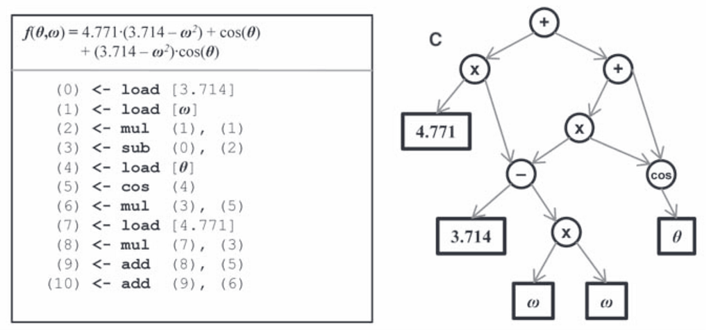
The first method which deserves a mention is a seminal work by Schmidt and Lipson which used Genetic Programming (GP) for symbolic regression and extracted equation from data of trajectories of simple dynamical systems such as double pendulum etc. The procedure consists of generating candidate symbolic functions, derive partial derivatives involved in these expressions and compare them with numerically estimated derivatives from data. Procedure is repeated until sufficient accuracy is reached. Importantly, as there is a very large number of potential candidate expressions which are relatively accurate, one choses the ones which satisfy the principle of “parsimony”. Parsimony is measured as the inverse of the number of terms in the expression, whereas the predictive accuracy is measured as the error on withheld experimental data used only for validation. This principle of parsimonious modelling forms the bedrock of equation discovery.
This method has the advantage of exploring various possible combinations of analytical expressions. It has been tried in various systems, in particular, I will highlight AI — Feynman which with the help of GP and neural networks allowed to identify from data 100 equations from Feynman lectures on physics. Another interesting application of GP is discovering ocean parameterisations in climate, where essentially a higher fidelity model is run to provide the training data, while a correction for cheaper lower fidelity model is discovered from the training data. With that being said, GP is not without its faults and human-in-the-loop was indispensable to ensure that the parameterisations work well. In addition, it can be very inefficient because it follows the recipe of evolution: trial and error. Are there other possibilities? This brings us to the method which has dominated the field of equation discovery in the recent years.
Sparse system identification
Sparse Identification of Nonlinear Dynamics (SINDy) belongs to the family of conceptually simple yet powerful methods. It was introduced by the group of Steven L. Brunton alongside other groups and is supplied with well-documented, well-supported repository and youtube tutorials. To get some practical hands-on experience just try out their Jupyter notebooks.
https://medium.com/media/eb0bb08b35d81427dd1b89c5699f1711/href
I will describe the method following the original SINDy paper. Typically, one has the trajectory data, which consists of coordinates such as x(t), y(t), z(t), etc. The goal is to reconstruct first-order Ordinary Differential Equations (ODEs) from data:


Finite difference method (for example) is typically used to compute the derivatives on the left hand side of the ODE. Because derivative estimation is prone to error this generates noise in the data which is generally unwanted. In some cases, filtering may help to deal with these problems. Next, a library of monomials (basis functions) is chosen to fit the right hand side of the ODEs as described in the graphic:

The problem is that unless we were in possession of astronomical amounts of data, this task would be hopeless, since many different polynomials would work just fine which would lead to spectacular overfitting. Fortunately, this is where sparse regression comes to rescue: the point is to penalise having too many active basis functions on the right hand side. This can be done in many ways. One of the methods on which the original SINDy relied on is called Sequential Threshold Least Squares (STLS) which can be summarised as follows:

In other words, solve for the coefficients using standard least squares method and then eliminate the small coefficients sequentially while applying the least squares each time. The procedure relies on a hyperparameter which controls the tolerance for the smallness of the coefficients. This parameter appears arbitrary, however, one may perform what is known as Pareto analysis: determine this sparsification hyperparameter by holding out some data and testing how well the learned model performs on the test set. The reasonable value for this coefficient corresponds to the “elbow’’ in the curve of the accuracy vs complexity of the learned model (complexity = how many terms it includes), the so-called Pareto front. Alternatively, some other publications have promoted sparsity using information criteria instead of performing Pareto analysis described above.
As a simplest application of SINDy, consider how STLS can be used to successfully identify Lorenz 63 model from data:

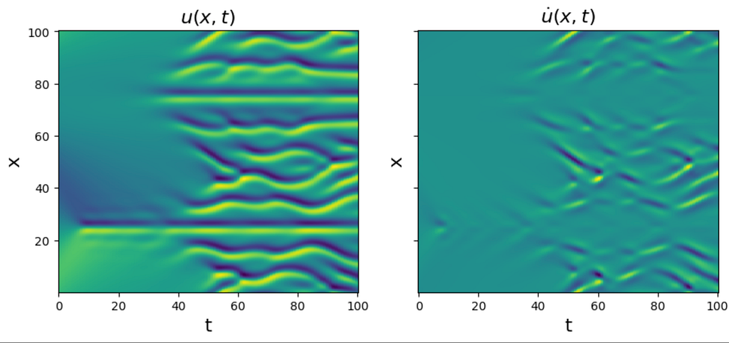
The STLS has limitations when applied to the large number of degree of freedom systems such as Partial Differential Equations (PDEs) and in this case one may consider dimensional reduction through Principal Component Analysis (PCA) or nonlinear autoencoders etc. Later the the SINDy algorithm was further imporoved by PDE-FIND paper which introduced Sequential Threshold Ridge (STRidge). In the latter ridge regression refers to regression with L2 penalty and in STRidge it is alternated with elimination of small coefficients like in STLS. This allowed discovery of various standard PDEs from the simulation data such as Burgers’ equation, Korteweg–De Vries (KdV), Navier Stokes, Reaction-Diffusion and even a rather peculiar equation one often encounters in scientific machine learning called Kuramoto — Sivashinsky, which is generally tricky due to the need to estimate its fourth derivative term directly from data:

Identification of this equation happens directly from the following input data (which is obtained by numerically solving the same equation):
This is not to say that the method is error prone. In fact, one of the big challenges of applying SINDy to realistic observational data is that it tends to be sparse and noisy itself and usually identification suffers in such circumstances. The same issue also affects methods based on symbolic regression such as Genetic Programming (GP).
Weak SINDy is a more recent development which significantly improves the robustness of the algorithm with respect to the noise. This approach has been implemented independently by several authors, most notably by Daniel Messenger, Daniel R. Gurevich and Patrick Reinbold. The main idea is, rather than discovering differential form of the PDE, to discover its [weak] integral form by integrating the PDE over a set of domains multiplying it by some test functions. This allows integration by parts and thus removing tricky derivatives from the response function (unknown solution) of the PDE and instead applying these derivatives to the test functions which are known. The method was further implemented in plasma physics equation discovery carried out by Alves and Fiuza, where Vlasov equation and plasma fluid models were recovered from the simulation data.
Another, rather obvious, limitation of the SINDy approach is that identification is always restricted by the library of terms which form the basis, e.g. monomials. While, other types of basis functions can be used, such as trigonometric functions, this still not general enough. Suppose the PDE has a form of a rational function where both numerator and denominator could be polynomials:

This is the kind of situation that can be of course treated with Genetic Programming (GP) easily. However, SINDy was also extended to such situations introducing SINDy-PI (parallel-implicit), which was used successfully to identify PDE describing Belousov-Zhabotinsky reaction.
Finally, other sparsity promoting methods such as sparse Bayesian regression, also known as Relevance Vector Machine (RVM), were equally used to identify equations from data using precisely the same fitting the library of terms approach, but benefiting from marginalisation and “Occam’s razor” principles that are highly respected by statisticians. I am not covering these approaches here but it suffices to say that some authors such as Zhang and Lin have claimed more robust system identification of ODEs and this approach has been even tried for learning closures for simple baroclinic ocean models where the authors argued RVM appeared more robust than STRidge. In addition, these methods provide natural Uncertainty Quantification (UQ) for the estimated coefficients of the identified equation. With that being said, more recent developments of ensemble SINDy are more robust and provide UQ but rely instead on a statistical method of bootstrap aggregating (bagging) also widely applied in statistics and machine learning.
Physics informed deep learning identification
Alternative approach to both solving and identifying coefficients of PDEs which has attracted enormous attention in the literature concerns Physics Informed Neural Networks (PINNs). The main idea is to parametrise the solution of the PDE using a neural network and introduce the equation of motion or other types of physics-based inductive biases into the loss function. The loss function is evaluated on a pre-defined set of the so-called “collocation points”. When performing gradient descent, the weights of the neural network are adjusted and the solution is “learned”. The only data that needs to be provided includes initial and boundary conditions which are also penalised in a separate loss term. The method actually borrows from older collocation methods of solving PDEs that were not based on neural networks. The fact that neural networks provide a natural way of automatic differentiation makes this approach very attractive, however, as it turns out, PINNs are generally not competitive with standard numerical methods such as finite volumes/elements etc. Thus as a tool of solving the forward problem (solving the PDE numerically) PINNs are not so interesting.
They become interesting as a tool for solving inverse problems: estimating the model via the data, rather than generating data via a known model. In the original PINNs paper two unknown coefficients of Navier-Stokes equation are estimated from data

In retrospect, when comparing to algorithms such as PDE-FIND this seems rather naive, as the general form of the equation has already been assumed. Nevertheless, one interesting aspect of this work is that the algorithm is not fed the pressure, instead incompressible flow is assumed and the solution for the pressure is recovered directly by the PINN.
PINNs have been applied in all kinds of situations, one particular application I would like to highlight is space weather, where it was shown that their applications allows estimation of electron density in the radiation belts by solving inverse problem for Fokker-Planck equation. Here ensemble method (of re-training the neural network) turns out to be handy in estimating the uncertainty. Eventually, to achieve interpretability polynomial expansion of the learned diffusion coefficients is performed. It would certainly be interesting to compare this approach with using directly something like SINDy, that would also provude a polynomial expansion.
The term physics-informed has been taken up by other teams, who sometimes invented their own version of putting physics priors into neural nets and followed the formula of calling their approach something catchy like physics-based or physics-inspired etc. These approaches can sometimes be categorised as soft constraints (penalising not satisfying some equation or symmetry inside the loss) or hard constraints (implementing the constraints into the architecture of the neural network). Examples of such approaches can be found in climate science, for instance, among other disciplines.
Given the backpropagation of neural nets provide an alternative for estimating temporal and spatial derivatives, it seemed inevitable that the Sparse Regression (SR) or Genetic Programming (GP) would be coupled with these neural net collocation methods. While there are many of such studies, I will highlight one of them, DeePyMoD for relatively well-documented and supported repository. It is sufficient to understand how the method works to understand all the other studies that came around the same time or later and improve upon it in various ways.

The loss function consists of Mean Square Error (MSE):

and regularisation which promotes the functional form of the PDE

DeePyMoD is significantly more robust to noise even when compared to weak SINDy and requires only a fraction of observation points on the spatio-temporal domain which is great news for discovering equations from observational data. For instance, many of the standard PDEs that PDE-FIND gets right can also be identified by DeePyMoD but only sampling on the order of few thousand points in space incorporating noise dominated data. However, using neural networks for this task comes at a cost of longer convergence. Another issue is that some PDEs are problematic for the vanilla collocation methods, for instance the Kuramoto-Sivashinsky (KS) equation due its high order derivatives. KS is generally hard to identify from data without weak-form approaches, especially in the presence of noise. More recent developments to aid this problem involve coupling weak SINDy approach with neural network collocation methods. Another interesting, practically unexplored question is how such methods are generally affected by non-Gaussian noise.
Conclusion
To summarise, equation discovery is a natural candidate for physics-based machine learning, which is being actively developed by various groups in the world. It has found applications in many fields such as fluid dynamics, plasma physics, climate and beyond. For a broader overview with the emphasis on some other methods see the review article. Hopefully, the reader got a flavour of different methodologies which exist in the field, but I have only scratched the surface by avoiding getting too technical. It is important to mention many new approaches to physics-based machine learning such as neural Ordinary Differential Equations (ODEs).
Bibliography
- Camps-Valls, G. et al. Discovering causal relations and equations from data. Physics Reports 1044, 1–68 (2023).
- Lam, R. et al. Learning skillful medium-range global weather forecasting. Science 0, eadi2336 (2023).
- Mehta, P. et al. A high-bias, low-variance introduction to Machine Learning for physicists. Physics Reports 810, 1–124 (2019).
- Schmidt, M. & Lipson, H. Distilling Free-Form Natural Laws from Experimental Data. Science 324, 81–85 (2009).
- Udrescu, S.-M. & Tegmark, M. AI Feynman: A physics-inspired method for symbolic regression. Sci Adv 6, eaay2631 (2020).
- Ross, A., Li, Z., Perezhogin, P., Fernandez-Granda, C. & Zanna, L. Benchmarking of Machine Learning Ocean Subgrid Parameterizations in an Idealized Model. Journal of Advances in Modeling Earth Systems 15, e2022MS003258 (2023).
- Brunton, S. L., Proctor, J. L. & Kutz, J. N. Discovering governing equations from data by sparse identification of nonlinear dynamical systems. Proceedings of the National Academy of Sciences 113, 3932–3937 (2016).
- Mangan, N. M., Kutz, J. N., Brunton, S. L. & Proctor, J. L. Model selection for dynamical systems via sparse regression and information criteria. Proceedings of the Royal Society A: Mathematical, Physical and Engineering Sciences 473, 20170009 (2017).
- Rudy, S. H., Brunton, S. L., Proctor, J. L. & Kutz, J. N. Data-driven discovery of partial differential equations. Science Advances 3, e1602614 (2017).
- Messenger, D. A. & Bortz, D. M. Weak SINDy for partial differential equations. Journal of Computational Physics 443, 110525 (2021).
- Gurevich, D. R., Reinbold, P. A. K. & Grigoriev, R. O. Robust and optimal sparse regression for nonlinear PDE models. Chaos: An Interdisciplinary Journal of Nonlinear Science 29, 103113 (2019).
- Reinbold, P. A. K., Kageorge, L. M., Schatz, M. F. & Grigoriev, R. O. Robust learning from noisy, incomplete, high-dimensional experimental data via physically constrained symbolic regression. Nat Commun 12, 3219 (2021).
- Alves, E. P. & Fiuza, F. Data-driven discovery of reduced plasma physics models from fully kinetic simulations. Phys. Rev. Res. 4, 033192 (2022).
- Zhang, S. & Lin, G. Robust data-driven discovery of governing physical laws with error bars. Proceedings of the Royal Society A: Mathematical, Physical and Engineering Sciences 474, 20180305 (2018).
- Zanna, L. & Bolton, T. Data-Driven Equation Discovery of Ocean Mesoscale Closures. Geophysical Research Letters 47, e2020GL088376 (2020).
- Fasel, U., Kutz, J. N., Brunton, B. W. & Brunton, S. L. Ensemble-SINDy: Robust sparse model discovery in the low-data, high-noise limit, with active learning and control. Proceedings of the Royal Society A: Mathematical, Physical and Engineering Sciences 478, 20210904 (2022).
- Raissi, M., Perdikaris, P. & Karniadakis, G. E. Physics-informed neural networks: A deep learning framework for solving forward and inverse problems involving nonlinear partial differential equations. Journal of Computational Physics 378, 686–707 (2019).
- Markidis, S. The Old and the New: Can Physics-Informed Deep-Learning Replace Traditional Linear Solvers? Frontiers in Big Data 4, (2021).
- Camporeale, E., Wilkie, G. J., Drozdov, A. Y. & Bortnik, J. Data-Driven Discovery of Fokker-Planck Equation for the Earth’s Radiation Belts Electrons Using Physics-Informed Neural Networks. Journal of Geophysical Research: Space Physics 127, e2022JA030377 (2022).
- Beucler, T. et al. Enforcing Analytic Constraints in Neural Networks Emulating Physical Systems. Phys. Rev. Lett. 126, 098302 (2021).
- Both, G.-J., Choudhury, S., Sens, P. & Kusters, R. DeepMoD: Deep learning for model discovery in noisy data. Journal of Computational Physics 428, 109985 (2021).
- Stephany, R. & Earls, C. PDE-READ: Human-readable partial differential equation discovery using deep learning. Neural Networks 154, 360–382 (2022).
- Both, G.-J., Vermarien, G. & Kusters, R. Sparsely constrained neural networks for model discovery of PDEs. Preprint at https://doi.org/10.48550/arXiv.2011.04336 (2021).
- Stephany, R. & Earls, C. Weak-PDE-LEARN: A Weak Form Based Approach to Discovering PDEs From Noisy, Limited Data. Preprint at https://doi.org/10.48550/arXiv.2309.04699 (2023).
On Data-Driven Equation Discovery was originally published in Towards Data Science on Medium, where people are continuing the conversation by highlighting and responding to this story.

Describing the nature with the help of analytical expressions verified through experiments has been a hallmark of the success of science especially in physics from fundamental law of gravitation to quantum mechanics and beyond. As challenges such as climate change, fusion, and computational biology pivot our focus toward more compute, there is a growing need for concise yet robust reduced models that maintain physical consistency at a lower cost. Scientific machine learning is an emergent field which promises to provide such solutions. This article is a short review of recent data-driven equation discovery methods targeting scientists and engineers familiar with very basics of machine learning or statistics.
Motivation and historical perspectives
Simply fitting the data well has proven to be a short-sighted endeavour, as demonstrated by the Ptolemy’s model of geocentrism which was the most observationally accurate model until Kepler’s heliocentric one. Thus, combining observations with fundamental physical principles plays a big role in science. However, often in physics we forget the extent to which our models of the world are already data driven. Take an example of standard model of particles with 19 parameters, whose numerical values are established by experiment. Earth system models used for meteorology and climate, while running on a physically consistent core based on fluid dynamics, also require careful calibration to observations of many of their sensitive parameters. Finally, reduced order modelling is gaining traction in fusion and space weather community and will likely remain relevant in future. In fields such as biology and social sciences, where first principle approaches are less effective, statistical system identification already plays a significant role.
There are various methods in machine learning that allow predicting the evolution of the system directly from data. More recently, deep neural networks have achieved significant advances in the field of weather forecasting as demonstrated by the team of Google’s DeepMind and others. This is partly due to the enormous resources available to them as well as general availability of meteorological data and physical numerical weather prediction models which have interpolated this data over the whole globe thanks to data assimilation. However, if the conditions under which data has been generated change (such as climate change) there is a risk that such fully-data driven models would poorly generalise. This means that applying such black box approaches to climate modelling and other situations where we have lack of data could be suspect. Thus, in this article I will emphasise methods which extract equation from data, since equations are more interpretable and suffer less from overfitting. In machine learning speak we can refer to such paradigms as high bias — low variance.
The first method which deserves a mention is a seminal work by Schmidt and Lipson which used Genetic Programming (GP) for symbolic regression and extracted equation from data of trajectories of simple dynamical systems such as double pendulum etc. The procedure consists of generating candidate symbolic functions, derive partial derivatives involved in these expressions and compare them with numerically estimated derivatives from data. Procedure is repeated until sufficient accuracy is reached. Importantly, as there is a very large number of potential candidate expressions which are relatively accurate, one choses the ones which satisfy the principle of “parsimony”. Parsimony is measured as the inverse of the number of terms in the expression, whereas the predictive accuracy is measured as the error on withheld experimental data used only for validation. This principle of parsimonious modelling forms the bedrock of equation discovery.
This method has the advantage of exploring various possible combinations of analytical expressions. It has been tried in various systems, in particular, I will highlight AI — Feynman which with the help of GP and neural networks allowed to identify from data 100 equations from Feynman lectures on physics. Another interesting application of GP is discovering ocean parameterisations in climate, where essentially a higher fidelity model is run to provide the training data, while a correction for cheaper lower fidelity model is discovered from the training data. With that being said, GP is not without its faults and human-in-the-loop was indispensable to ensure that the parameterisations work well. In addition, it can be very inefficient because it follows the recipe of evolution: trial and error. Are there other possibilities? This brings us to the method which has dominated the field of equation discovery in the recent years.
Sparse system identification
Sparse Identification of Nonlinear Dynamics (SINDy) belongs to the family of conceptually simple yet powerful methods. It was introduced by the group of Steven L. Brunton alongside other groups and is supplied with well-documented, well-supported repository and youtube tutorials. To get some practical hands-on experience just try out their Jupyter notebooks.
https://medium.com/media/eb0bb08b35d81427dd1b89c5699f1711/href
I will describe the method following the original SINDy paper. Typically, one has the trajectory data, which consists of coordinates such as x(t), y(t), z(t), etc. The goal is to reconstruct first-order Ordinary Differential Equations (ODEs) from data:
Finite difference method (for example) is typically used to compute the derivatives on the left hand side of the ODE. Because derivative estimation is prone to error this generates noise in the data which is generally unwanted. In some cases, filtering may help to deal with these problems. Next, a library of monomials (basis functions) is chosen to fit the right hand side of the ODEs as described in the graphic:
The problem is that unless we were in possession of astronomical amounts of data, this task would be hopeless, since many different polynomials would work just fine which would lead to spectacular overfitting. Fortunately, this is where sparse regression comes to rescue: the point is to penalise having too many active basis functions on the right hand side. This can be done in many ways. One of the methods on which the original SINDy relied on is called Sequential Threshold Least Squares (STLS) which can be summarised as follows:
In other words, solve for the coefficients using standard least squares method and then eliminate the small coefficients sequentially while applying the least squares each time. The procedure relies on a hyperparameter which controls the tolerance for the smallness of the coefficients. This parameter appears arbitrary, however, one may perform what is known as Pareto analysis: determine this sparsification hyperparameter by holding out some data and testing how well the learned model performs on the test set. The reasonable value for this coefficient corresponds to the “elbow’’ in the curve of the accuracy vs complexity of the learned model (complexity = how many terms it includes), the so-called Pareto front. Alternatively, some other publications have promoted sparsity using information criteria instead of performing Pareto analysis described above.
As a simplest application of SINDy, consider how STLS can be used to successfully identify Lorenz 63 model from data:
The STLS has limitations when applied to the large number of degree of freedom systems such as Partial Differential Equations (PDEs) and in this case one may consider dimensional reduction through Principal Component Analysis (PCA) or nonlinear autoencoders etc. Later the the SINDy algorithm was further imporoved by PDE-FIND paper which introduced Sequential Threshold Ridge (STRidge). In the latter ridge regression refers to regression with L2 penalty and in STRidge it is alternated with elimination of small coefficients like in STLS. This allowed discovery of various standard PDEs from the simulation data such as Burgers’ equation, Korteweg–De Vries (KdV), Navier Stokes, Reaction-Diffusion and even a rather peculiar equation one often encounters in scientific machine learning called Kuramoto — Sivashinsky, which is generally tricky due to the need to estimate its fourth derivative term directly from data:
Identification of this equation happens directly from the following input data (which is obtained by numerically solving the same equation):
This is not to say that the method is error prone. In fact, one of the big challenges of applying SINDy to realistic observational data is that it tends to be sparse and noisy itself and usually identification suffers in such circumstances. The same issue also affects methods based on symbolic regression such as Genetic Programming (GP).
Weak SINDy is a more recent development which significantly improves the robustness of the algorithm with respect to the noise. This approach has been implemented independently by several authors, most notably by Daniel Messenger, Daniel R. Gurevich and Patrick Reinbold. The main idea is, rather than discovering differential form of the PDE, to discover its [weak] integral form by integrating the PDE over a set of domains multiplying it by some test functions. This allows integration by parts and thus removing tricky derivatives from the response function (unknown solution) of the PDE and instead applying these derivatives to the test functions which are known. The method was further implemented in plasma physics equation discovery carried out by Alves and Fiuza, where Vlasov equation and plasma fluid models were recovered from the simulation data.
Another, rather obvious, limitation of the SINDy approach is that identification is always restricted by the library of terms which form the basis, e.g. monomials. While, other types of basis functions can be used, such as trigonometric functions, this still not general enough. Suppose the PDE has a form of a rational function where both numerator and denominator could be polynomials:
This is the kind of situation that can be of course treated with Genetic Programming (GP) easily. However, SINDy was also extended to such situations introducing SINDy-PI (parallel-implicit), which was used successfully to identify PDE describing Belousov-Zhabotinsky reaction.
Finally, other sparsity promoting methods such as sparse Bayesian regression, also known as Relevance Vector Machine (RVM), were equally used to identify equations from data using precisely the same fitting the library of terms approach, but benefiting from marginalisation and “Occam’s razor” principles that are highly respected by statisticians. I am not covering these approaches here but it suffices to say that some authors such as Zhang and Lin have claimed more robust system identification of ODEs and this approach has been even tried for learning closures for simple baroclinic ocean models where the authors argued RVM appeared more robust than STRidge. In addition, these methods provide natural Uncertainty Quantification (UQ) for the estimated coefficients of the identified equation. With that being said, more recent developments of ensemble SINDy are more robust and provide UQ but rely instead on a statistical method of bootstrap aggregating (bagging) also widely applied in statistics and machine learning.
Physics informed deep learning identification
Alternative approach to both solving and identifying coefficients of PDEs which has attracted enormous attention in the literature concerns Physics Informed Neural Networks (PINNs). The main idea is to parametrise the solution of the PDE using a neural network and introduce the equation of motion or other types of physics-based inductive biases into the loss function. The loss function is evaluated on a pre-defined set of the so-called “collocation points”. When performing gradient descent, the weights of the neural network are adjusted and the solution is “learned”. The only data that needs to be provided includes initial and boundary conditions which are also penalised in a separate loss term. The method actually borrows from older collocation methods of solving PDEs that were not based on neural networks. The fact that neural networks provide a natural way of automatic differentiation makes this approach very attractive, however, as it turns out, PINNs are generally not competitive with standard numerical methods such as finite volumes/elements etc. Thus as a tool of solving the forward problem (solving the PDE numerically) PINNs are not so interesting.
They become interesting as a tool for solving inverse problems: estimating the model via the data, rather than generating data via a known model. In the original PINNs paper two unknown coefficients of Navier-Stokes equation are estimated from data
In retrospect, when comparing to algorithms such as PDE-FIND this seems rather naive, as the general form of the equation has already been assumed. Nevertheless, one interesting aspect of this work is that the algorithm is not fed the pressure, instead incompressible flow is assumed and the solution for the pressure is recovered directly by the PINN.
PINNs have been applied in all kinds of situations, one particular application I would like to highlight is space weather, where it was shown that their applications allows estimation of electron density in the radiation belts by solving inverse problem for Fokker-Planck equation. Here ensemble method (of re-training the neural network) turns out to be handy in estimating the uncertainty. Eventually, to achieve interpretability polynomial expansion of the learned diffusion coefficients is performed. It would certainly be interesting to compare this approach with using directly something like SINDy, that would also provude a polynomial expansion.
The term physics-informed has been taken up by other teams, who sometimes invented their own version of putting physics priors into neural nets and followed the formula of calling their approach something catchy like physics-based or physics-inspired etc. These approaches can sometimes be categorised as soft constraints (penalising not satisfying some equation or symmetry inside the loss) or hard constraints (implementing the constraints into the architecture of the neural network). Examples of such approaches can be found in climate science, for instance, among other disciplines.
Given the backpropagation of neural nets provide an alternative for estimating temporal and spatial derivatives, it seemed inevitable that the Sparse Regression (SR) or Genetic Programming (GP) would be coupled with these neural net collocation methods. While there are many of such studies, I will highlight one of them, DeePyMoD for relatively well-documented and supported repository. It is sufficient to understand how the method works to understand all the other studies that came around the same time or later and improve upon it in various ways.
The loss function consists of Mean Square Error (MSE):
and regularisation which promotes the functional form of the PDE
DeePyMoD is significantly more robust to noise even when compared to weak SINDy and requires only a fraction of observation points on the spatio-temporal domain which is great news for discovering equations from observational data. For instance, many of the standard PDEs that PDE-FIND gets right can also be identified by DeePyMoD but only sampling on the order of few thousand points in space incorporating noise dominated data. However, using neural networks for this task comes at a cost of longer convergence. Another issue is that some PDEs are problematic for the vanilla collocation methods, for instance the Kuramoto-Sivashinsky (KS) equation due its high order derivatives. KS is generally hard to identify from data without weak-form approaches, especially in the presence of noise. More recent developments to aid this problem involve coupling weak SINDy approach with neural network collocation methods. Another interesting, practically unexplored question is how such methods are generally affected by non-Gaussian noise.
Conclusion
To summarise, equation discovery is a natural candidate for physics-based machine learning, which is being actively developed by various groups in the world. It has found applications in many fields such as fluid dynamics, plasma physics, climate and beyond. For a broader overview with the emphasis on some other methods see the review article. Hopefully, the reader got a flavour of different methodologies which exist in the field, but I have only scratched the surface by avoiding getting too technical. It is important to mention many new approaches to physics-based machine learning such as neural Ordinary Differential Equations (ODEs).
Bibliography
- Camps-Valls, G. et al. Discovering causal relations and equations from data. Physics Reports 1044, 1–68 (2023).
- Lam, R. et al. Learning skillful medium-range global weather forecasting. Science 0, eadi2336 (2023).
- Mehta, P. et al. A high-bias, low-variance introduction to Machine Learning for physicists. Physics Reports 810, 1–124 (2019).
- Schmidt, M. & Lipson, H. Distilling Free-Form Natural Laws from Experimental Data. Science 324, 81–85 (2009).
- Udrescu, S.-M. & Tegmark, M. AI Feynman: A physics-inspired method for symbolic regression. Sci Adv 6, eaay2631 (2020).
- Ross, A., Li, Z., Perezhogin, P., Fernandez-Granda, C. & Zanna, L. Benchmarking of Machine Learning Ocean Subgrid Parameterizations in an Idealized Model. Journal of Advances in Modeling Earth Systems 15, e2022MS003258 (2023).
- Brunton, S. L., Proctor, J. L. & Kutz, J. N. Discovering governing equations from data by sparse identification of nonlinear dynamical systems. Proceedings of the National Academy of Sciences 113, 3932–3937 (2016).
- Mangan, N. M., Kutz, J. N., Brunton, S. L. & Proctor, J. L. Model selection for dynamical systems via sparse regression and information criteria. Proceedings of the Royal Society A: Mathematical, Physical and Engineering Sciences 473, 20170009 (2017).
- Rudy, S. H., Brunton, S. L., Proctor, J. L. & Kutz, J. N. Data-driven discovery of partial differential equations. Science Advances 3, e1602614 (2017).
- Messenger, D. A. & Bortz, D. M. Weak SINDy for partial differential equations. Journal of Computational Physics 443, 110525 (2021).
- Gurevich, D. R., Reinbold, P. A. K. & Grigoriev, R. O. Robust and optimal sparse regression for nonlinear PDE models. Chaos: An Interdisciplinary Journal of Nonlinear Science 29, 103113 (2019).
- Reinbold, P. A. K., Kageorge, L. M., Schatz, M. F. & Grigoriev, R. O. Robust learning from noisy, incomplete, high-dimensional experimental data via physically constrained symbolic regression. Nat Commun 12, 3219 (2021).
- Alves, E. P. & Fiuza, F. Data-driven discovery of reduced plasma physics models from fully kinetic simulations. Phys. Rev. Res. 4, 033192 (2022).
- Zhang, S. & Lin, G. Robust data-driven discovery of governing physical laws with error bars. Proceedings of the Royal Society A: Mathematical, Physical and Engineering Sciences 474, 20180305 (2018).
- Zanna, L. & Bolton, T. Data-Driven Equation Discovery of Ocean Mesoscale Closures. Geophysical Research Letters 47, e2020GL088376 (2020).
- Fasel, U., Kutz, J. N., Brunton, B. W. & Brunton, S. L. Ensemble-SINDy: Robust sparse model discovery in the low-data, high-noise limit, with active learning and control. Proceedings of the Royal Society A: Mathematical, Physical and Engineering Sciences 478, 20210904 (2022).
- Raissi, M., Perdikaris, P. & Karniadakis, G. E. Physics-informed neural networks: A deep learning framework for solving forward and inverse problems involving nonlinear partial differential equations. Journal of Computational Physics 378, 686–707 (2019).
- Markidis, S. The Old and the New: Can Physics-Informed Deep-Learning Replace Traditional Linear Solvers? Frontiers in Big Data 4, (2021).
- Camporeale, E., Wilkie, G. J., Drozdov, A. Y. & Bortnik, J. Data-Driven Discovery of Fokker-Planck Equation for the Earth’s Radiation Belts Electrons Using Physics-Informed Neural Networks. Journal of Geophysical Research: Space Physics 127, e2022JA030377 (2022).
- Beucler, T. et al. Enforcing Analytic Constraints in Neural Networks Emulating Physical Systems. Phys. Rev. Lett. 126, 098302 (2021).
- Both, G.-J., Choudhury, S., Sens, P. & Kusters, R. DeepMoD: Deep learning for model discovery in noisy data. Journal of Computational Physics 428, 109985 (2021).
- Stephany, R. & Earls, C. PDE-READ: Human-readable partial differential equation discovery using deep learning. Neural Networks 154, 360–382 (2022).
- Both, G.-J., Vermarien, G. & Kusters, R. Sparsely constrained neural networks for model discovery of PDEs. Preprint at https://doi.org/10.48550/arXiv.2011.04336 (2021).
- Stephany, R. & Earls, C. Weak-PDE-LEARN: A Weak Form Based Approach to Discovering PDEs From Noisy, Limited Data. Preprint at https://doi.org/10.48550/arXiv.2309.04699 (2023).
On Data-Driven Equation Discovery was originally published in Towards Data Science on Medium, where people are continuing the conversation by highlighting and responding to this story.
Denial of responsibility! Techno Blender is an automatic aggregator of the all world’s media. In each content, the hyperlink to the primary source is specified. All trademarks belong to their rightful owners, all materials to their authors. If you are the owner of the content and do not want us to publish your materials, please contact us by email – [email protected]. The content will be deleted within 24 hours.