
On the statistical analysis of rounded or binned data
On the Statistical Analysis of Rounded or Binned Data
Sheppard’s corrections offer approximations, but errors persist. Analytical bounds provide insight into the magnitude of these errors
Imagine having a list of length measurements in inches, precise to the inch. This list might represent, for instance, the heights of individuals participating in a medical study, forming a sample from a cohort of interest. Our goal is to estimate the average height within this cohort.
Consider an arithmetic mean of 70.08 inches. The crucial question is: How accurate is this figure? Despite a large sample size, the reality is that each individual measurement is only precise up to the inch. Thus, even with abundant data, we might cautiously assume that the true average height falls within the range of 69.5 inches to 70.5 inches, and round the value to 70 inches.
This isn’t merely a theoretical concern easily dismissed. Take, for instance, determining the average height in metric units. One inch equals exactly 2.54 centimeters, so we can easily convert the measurements from inches to the finer centimeter scale, and compute the mean. Yet, considering the inch-level accuracy, we can only confidently assert that the average height lies somewhere between 177 cm and 179 cm. The question arises: Can we confidently conclude that the average height is precisely 178 cm?
Rounding errors or quantization errors can have enormous consequences— such as changing the outcome of elections, or changing the course of a ballistic missile, leading to accidental death and injury. How rounding errors affect statistical analyses is a non-trivial inquiry that we aim to elucidate in this article.
Sheppard’s corrections
Suppose that we observe values produced by a continuous random variable X that have been rounded, or binned. These observations follow the distribution of a discrete random variable Y defined by:

where h is the bin width and ⌊ ⋅ ⌋ denotes the floor function. For example, X could generate length measurements. Since rounding is not an invertible operation, reconstructing the original data from the rounded values alone is impossible.
The following approximations relate the mean and the variance of these distributions, known as Sheppard’s corrections [Sheppard 1897]:

For example, if we are given measurements rounded to the inch, h = 2.54 cm, and observe a standard deviation of 10.0 cm, Sheppard’s second moment correction asks us to assume that the original data have in fact a smaller standard deviation of σ = 9.97 cm. For many practical purposes, the correction is very small. Even if the standard deviation is of similar magnitude as the bin width, the correction only amounts to 5% of the original value.
Sheppard’s corrections can be applied if the following conditions hold [Kendall 1938, Heitjan 1989]:
- the probability density function of X is sufficiently smooth and its derivatives tend to zero at its tails,
- the bin width h is not too large (h < 1.6 σ),
- the sample size N is not too small and not too large (5 < N < 100).
The first two requirements present as the typical “no free lunch” situation in statistical inference: in order to check whether these conditions hold, we would have to know the true distribution in the first place. The first of these conditions, in particular, is a local condition in the sense that it involves derivatives of the density which we cannot robustly estimate given only the rounded or binned data.
The requirement on the sample size not being too large does not mean that the propagation of rounding errors becomes less controllable (in absolute value) with large sample size. Instead, it addresses the situation where Sheppard’s corrections may cease to be adequate when attempting to compare the bias introduced by rounding/binning with the diminishing standard error in larger samples.
Total variation bounds on the rounding error in estimating the mean
Sheppard’s corrections are only approximations. For example, in general, the bias in estimating the mean, E[Y] – E[X], is in fact non-zero. We want to compute some upper bounds on the absolute value of this bias. The simplest bound is a result of the monotonicity of the expected value, and the fact that rounding/binning can change the values by at most h / 2:

With no additional information on the distribution of X available, we are not able to improve on this bound: imagine that the probability mass of X is highly concentrated just above the midpoint of a bin, then all values produced by X will be shifted by + h / 2 to result in a value for Y, realizing the upper bound.
However, the following exact formula can be given, based on [Theorem 2.3 (i), Svante 2005]:

Here, φ( ⋅ ) denotes the characteristic function of X, i.e., the Fourier transform of the unknown probability density function p( ⋅ ). This formula implies the following bound:

We can calculate this bound for some of our favorite distributions, for example the uniform distribution with support on the interval [a, b]:
Here, we have used the well-known value of the sum of reciprocals of squares. For example, if we sample from a uniform distribution with range b – a = 10 cm, and compute the mean from data that has been rounded to a precision of h = 2.54 cm, the bias in estimating the mean is at most 1.1 millimeters.
By a calculation very similar to one performed in [Ushakov & Ushakov 2022], we may also bound the rounding error when sampling from a normal distribution with variance σ²:
The exponential term decays very fast with smaller values of the bin width. For example, given a standard deviation of σ = 10 cm and a bin width of h = 2.54 cm the rounding error in estimating the mean is of the order 10^(-133), i.e., it is negligible for any practical purpose.
Applying Theorem 2.5.3 of [Ushakov 1999], we can give a more general bound in terms of the total variation V(p) of the probability density function p( ⋅ ) instead of its characteristic function:

where

The calculation is similar to one provided in [Ushakov & Ushakov 2018]. For example, the total variation of the uniform distribution with support on the interval [a, b] is given by 2 / (b – a), so the above formula provides the same bound as the previous calculation, via the modulus of the characteristic function.
The total variation bound allows us to provide a formula for practical use that estimates an upper bound for the rounding error, based on the histogram with bin width h:

Here, n_k is the number of observations that fall into the k-th bin.
As a numerical example, we analyze N = 412,659 of person’s height values surveyed by the U.S. Centers for Disease Control and Prevention [CDC 2022], given in inches. The mean height in metric units is given by 170.33 cm. Because of the large sample size, the standard error σ / √N is very small, 0.02 cm. However, the error due to rounding may be larger, as the total variation bound can be estimated to be 0.05 cm. In this case, the statistical errors are negligible since differences in body height well below a centimeter are rarely of practical relevance. For other cases that require highly accurate estimates of the average value of measurements, however, it may not be sufficient to just compute the standard error when the data is subject to quantization.
Bounds based on Fisher information
If the probability density function p( ⋅ ) is continuously differentiable, we can express its total variation V(p) as an integral over the derivatives’ modulus. Applying Hölder’s inequality, we can bound the total variation by (the square root of) the Fisher information I(p):
Consequently, we can write down an additional upper bound to the bias when computing the mean of rounded or binned data:

This new bound is of (theoretical) interest since Fisher information is a characteristic of the density function that is more commonly used than its total variation.
More bounds can be found via known upper bounds for the Fisher information, many of which can be found in [Bobkov 2022], including the following involving the third derivative of the probability density function:

Curiously, Fisher information also holds significance in certain formulations of quantum mechanics, wherein it serves as the component of the Hamiltonian responsible for inducing quantum effects [Curcuraci & Ramezani 2019]. One might ponder the existence of a concrete and meaningful link between quantized physical matter and classical measurements subjected to “ordinary” quantization. However, it is important to note that such speculation is likely rooted in mathematical pareidolia.
Conclusion
Sheppard’s corrections are approximations that can be used to account for errors in computing the mean, variance, and other (central) moments of a distribution based on rounded or binned data.
Although Sheppard’s correction for the mean is zero, the actual error may be comparable to, or even exceed, the standard error, especially for larger samples. We can constrain the error in computing the mean based on rounded or binned data by considering the total variation of the probability density function, a quantity estimable from the binned data.
Additional bounds on the rounding error when estimating the mean can be expressed in terms of the Fisher information and higher derivatives of the probability density function of the unknown distribution.
References
[Sheppard 1897] Sheppard, W.F. (1897). “On the Calculation of the most Probable Values of Frequency-Constants, for Data arranged according to Equidistant Division of a Scale.” Proceedings of the London Mathematical Society s1–29: 353–380.
[Kendall 1938] Kendall, M. G. (1938). “The Conditions under which Sheppard’s Corrections are Valid.” Journal of the Royal Statistical Society 101(3): 592–605.
[Heitjan 1989] Daniel F. Heitjan (1989). “Inference from Grouped Continuous Data: A Review.” Statist. Sci. 4 (2): 164–179.
[Svante 2005] Janson, Svante (2005). “Rounding of continuous random variables and oscillatory asymptotics.” Annals of Probability 34: 1807–1826.
[Ushakov & Ushakov 2022] Ushakov, N. G., & Ushakov, V. G. (2022). “On the effect of rounding on hypothesis testing when sample size is large.” Stat 11(1): e478.
[Ushakov 1999] Ushakov, N. G. (1999). “Selected Topics in Characteristic Functions.” De Gruyter.
[Ushakov & Ushakov 2018] Ushakov, N. G., Ushakov, V. G. Statistical Analysis of Rounded Data: Measurement Errors vs Rounding Errors. J Math Sci 234 (2018): 770–773.
[CDC 2022] Centers for Disease Control and Prevention (CDC). Behavioral Risk Factor Surveillance System Survey Data 2022. Atlanta, Georgia: U.S. Department of Health and Human Services, Centers for Disease Control and Prevention.
[Bobkov 2022] Bobkov, Sergey G. (2022). “Upper Bounds for Fisher information.” Electron. J. Probab. 27: 1–44.
[Curcuraci & Ramezani 2019] L. Curcuraci, M. Ramezani (2019). “A thermodynamical derivation of the quantum potential and the temperature of the wave function.” Physica A: Statistical Mechanics and its Applications 530: 121570.
On the statistical analysis of rounded or binned data was originally published in Towards Data Science on Medium, where people are continuing the conversation by highlighting and responding to this story.
On the Statistical Analysis of Rounded or Binned Data
Sheppard’s corrections offer approximations, but errors persist. Analytical bounds provide insight into the magnitude of these errors

Imagine having a list of length measurements in inches, precise to the inch. This list might represent, for instance, the heights of individuals participating in a medical study, forming a sample from a cohort of interest. Our goal is to estimate the average height within this cohort.
Consider an arithmetic mean of 70.08 inches. The crucial question is: How accurate is this figure? Despite a large sample size, the reality is that each individual measurement is only precise up to the inch. Thus, even with abundant data, we might cautiously assume that the true average height falls within the range of 69.5 inches to 70.5 inches, and round the value to 70 inches.
This isn’t merely a theoretical concern easily dismissed. Take, for instance, determining the average height in metric units. One inch equals exactly 2.54 centimeters, so we can easily convert the measurements from inches to the finer centimeter scale, and compute the mean. Yet, considering the inch-level accuracy, we can only confidently assert that the average height lies somewhere between 177 cm and 179 cm. The question arises: Can we confidently conclude that the average height is precisely 178 cm?
Rounding errors or quantization errors can have enormous consequences— such as changing the outcome of elections, or changing the course of a ballistic missile, leading to accidental death and injury. How rounding errors affect statistical analyses is a non-trivial inquiry that we aim to elucidate in this article.
Sheppard’s corrections
Suppose that we observe values produced by a continuous random variable X that have been rounded, or binned. These observations follow the distribution of a discrete random variable Y defined by:
where h is the bin width and ⌊ ⋅ ⌋ denotes the floor function. For example, X could generate length measurements. Since rounding is not an invertible operation, reconstructing the original data from the rounded values alone is impossible.
The following approximations relate the mean and the variance of these distributions, known as Sheppard’s corrections [Sheppard 1897]:
For example, if we are given measurements rounded to the inch, h = 2.54 cm, and observe a standard deviation of 10.0 cm, Sheppard’s second moment correction asks us to assume that the original data have in fact a smaller standard deviation of σ = 9.97 cm. For many practical purposes, the correction is very small. Even if the standard deviation is of similar magnitude as the bin width, the correction only amounts to 5% of the original value.
Sheppard’s corrections can be applied if the following conditions hold [Kendall 1938, Heitjan 1989]:
- the probability density function of X is sufficiently smooth and its derivatives tend to zero at its tails,
- the bin width h is not too large (h < 1.6 σ),
- the sample size N is not too small and not too large (5 < N < 100).
The first two requirements present as the typical “no free lunch” situation in statistical inference: in order to check whether these conditions hold, we would have to know the true distribution in the first place. The first of these conditions, in particular, is a local condition in the sense that it involves derivatives of the density which we cannot robustly estimate given only the rounded or binned data.
The requirement on the sample size not being too large does not mean that the propagation of rounding errors becomes less controllable (in absolute value) with large sample size. Instead, it addresses the situation where Sheppard’s corrections may cease to be adequate when attempting to compare the bias introduced by rounding/binning with the diminishing standard error in larger samples.
Total variation bounds on the rounding error in estimating the mean
Sheppard’s corrections are only approximations. For example, in general, the bias in estimating the mean, E[Y] – E[X], is in fact non-zero. We want to compute some upper bounds on the absolute value of this bias. The simplest bound is a result of the monotonicity of the expected value, and the fact that rounding/binning can change the values by at most h / 2:
With no additional information on the distribution of X available, we are not able to improve on this bound: imagine that the probability mass of X is highly concentrated just above the midpoint of a bin, then all values produced by X will be shifted by + h / 2 to result in a value for Y, realizing the upper bound.
However, the following exact formula can be given, based on [Theorem 2.3 (i), Svante 2005]:
Here, φ( ⋅ ) denotes the characteristic function of X, i.e., the Fourier transform of the unknown probability density function p( ⋅ ). This formula implies the following bound:
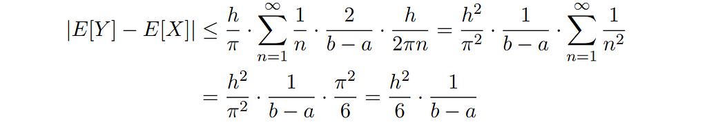
We can calculate this bound for some of our favorite distributions, for example the uniform distribution with support on the interval [a, b]:
Here, we have used the well-known value of the sum of reciprocals of squares. For example, if we sample from a uniform distribution with range b – a = 10 cm, and compute the mean from data that has been rounded to a precision of h = 2.54 cm, the bias in estimating the mean is at most 1.1 millimeters.
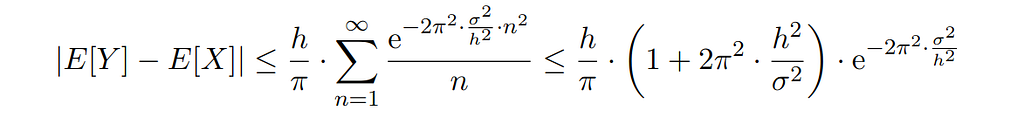
By a calculation very similar to one performed in [Ushakov & Ushakov 2022], we may also bound the rounding error when sampling from a normal distribution with variance σ²:
The exponential term decays very fast with smaller values of the bin width. For example, given a standard deviation of σ = 10 cm and a bin width of h = 2.54 cm the rounding error in estimating the mean is of the order 10^(-133), i.e., it is negligible for any practical purpose.
Applying Theorem 2.5.3 of [Ushakov 1999], we can give a more general bound in terms of the total variation V(p) of the probability density function p( ⋅ ) instead of its characteristic function:
where
The calculation is similar to one provided in [Ushakov & Ushakov 2018]. For example, the total variation of the uniform distribution with support on the interval [a, b] is given by 2 / (b – a), so the above formula provides the same bound as the previous calculation, via the modulus of the characteristic function.
The total variation bound allows us to provide a formula for practical use that estimates an upper bound for the rounding error, based on the histogram with bin width h:
Here, n_k is the number of observations that fall into the k-th bin.
As a numerical example, we analyze N = 412,659 of person’s height values surveyed by the U.S. Centers for Disease Control and Prevention [CDC 2022], given in inches. The mean height in metric units is given by 170.33 cm. Because of the large sample size, the standard error σ / √N is very small, 0.02 cm. However, the error due to rounding may be larger, as the total variation bound can be estimated to be 0.05 cm. In this case, the statistical errors are negligible since differences in body height well below a centimeter are rarely of practical relevance. For other cases that require highly accurate estimates of the average value of measurements, however, it may not be sufficient to just compute the standard error when the data is subject to quantization.
Bounds based on Fisher information
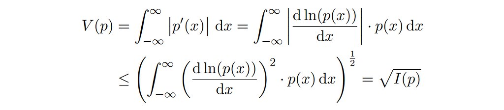
If the probability density function p( ⋅ ) is continuously differentiable, we can express its total variation V(p) as an integral over the derivatives’ modulus. Applying Hölder’s inequality, we can bound the total variation by (the square root of) the Fisher information I(p):
Consequently, we can write down an additional upper bound to the bias when computing the mean of rounded or binned data:
This new bound is of (theoretical) interest since Fisher information is a characteristic of the density function that is more commonly used than its total variation.
More bounds can be found via known upper bounds for the Fisher information, many of which can be found in [Bobkov 2022], including the following involving the third derivative of the probability density function:
Curiously, Fisher information also holds significance in certain formulations of quantum mechanics, wherein it serves as the component of the Hamiltonian responsible for inducing quantum effects [Curcuraci & Ramezani 2019]. One might ponder the existence of a concrete and meaningful link between quantized physical matter and classical measurements subjected to “ordinary” quantization. However, it is important to note that such speculation is likely rooted in mathematical pareidolia.
Conclusion
Sheppard’s corrections are approximations that can be used to account for errors in computing the mean, variance, and other (central) moments of a distribution based on rounded or binned data.
Although Sheppard’s correction for the mean is zero, the actual error may be comparable to, or even exceed, the standard error, especially for larger samples. We can constrain the error in computing the mean based on rounded or binned data by considering the total variation of the probability density function, a quantity estimable from the binned data.
Additional bounds on the rounding error when estimating the mean can be expressed in terms of the Fisher information and higher derivatives of the probability density function of the unknown distribution.
References
[Sheppard 1897] Sheppard, W.F. (1897). “On the Calculation of the most Probable Values of Frequency-Constants, for Data arranged according to Equidistant Division of a Scale.” Proceedings of the London Mathematical Society s1–29: 353–380.
[Kendall 1938] Kendall, M. G. (1938). “The Conditions under which Sheppard’s Corrections are Valid.” Journal of the Royal Statistical Society 101(3): 592–605.
[Heitjan 1989] Daniel F. Heitjan (1989). “Inference from Grouped Continuous Data: A Review.” Statist. Sci. 4 (2): 164–179.
[Svante 2005] Janson, Svante (2005). “Rounding of continuous random variables and oscillatory asymptotics.” Annals of Probability 34: 1807–1826.
[Ushakov & Ushakov 2022] Ushakov, N. G., & Ushakov, V. G. (2022). “On the effect of rounding on hypothesis testing when sample size is large.” Stat 11(1): e478.
[Ushakov 1999] Ushakov, N. G. (1999). “Selected Topics in Characteristic Functions.” De Gruyter.
[Ushakov & Ushakov 2018] Ushakov, N. G., Ushakov, V. G. Statistical Analysis of Rounded Data: Measurement Errors vs Rounding Errors. J Math Sci 234 (2018): 770–773.
[CDC 2022] Centers for Disease Control and Prevention (CDC). Behavioral Risk Factor Surveillance System Survey Data 2022. Atlanta, Georgia: U.S. Department of Health and Human Services, Centers for Disease Control and Prevention.
[Bobkov 2022] Bobkov, Sergey G. (2022). “Upper Bounds for Fisher information.” Electron. J. Probab. 27: 1–44.
[Curcuraci & Ramezani 2019] L. Curcuraci, M. Ramezani (2019). “A thermodynamical derivation of the quantum potential and the temperature of the wave function.” Physica A: Statistical Mechanics and its Applications 530: 121570.
On the statistical analysis of rounded or binned data was originally published in Towards Data Science on Medium, where people are continuing the conversation by highlighting and responding to this story.
Denial of responsibility! Techno Blender is an automatic aggregator of the all world’s media. In each content, the hyperlink to the primary source is specified. All trademarks belong to their rightful owners, all materials to their authors. If you are the owner of the content and do not want us to publish your materials, please contact us by email – [email protected]. The content will be deleted within 24 hours.