
Online Time Series Forecasting in Python | by Tyler Blume | Jul, 2022
An Example with ThymeBoost
Online learning involves updating parameters with new data without re-fitting the entire process. For models which involve boosting, such as ThymeBoost, the ability to pick up where we left off would save valuable computation time.
Luckily for us, the boosting procedure unlocks an easy path to updating parameters given new data. This is because the whole system is built to learn from residuals. Once we have new data, we simply need to predict for that new data and inject those residuals back into the procedure. The rest flows normally from there!
In this article, we will take a quick look at the new ‘update’ method for ThymeBoost which allows online learning to update the model as we receive new data.
For our example, we will generate a simple series which contains 2 trend-changepoints and some seasonality:
import numpy as np
import matplotlib.pyplot as plt
import seaborn as sns
import pandas as pd
sns.set_style('darkgrid')seasonality = ((np.cos(np.arange(1, 301))*10 + 50))
np.random.seed(100)
trend = np.linspace(-1, 1, 100)
trend = np.append(trend, np.linspace(1, 50, 100))
trend = np.append(trend, np.linspace(50, 1, 100))
y = trend + seasonality
plt.plot(y)
plt.show()

With our series in hand, let’s fit it with ThymeBoost the normal way. If you haven’t been exposed to ThymeBoost before, I recommend checking out this article which gives a good overview:
And make sure to have the most recent version from pip!
With that out of the way, let’s fit it:
from ThymeBoost import ThymeBoost as tb
boosted_model = tb.ThymeBoost(verbose=0,
n_rounds=None,
split_strategy='gradient')
output = boosted_model.fit(y,
min_sample_pct=.2,
trend_estimator=['linear'],
seasonal_estimator='fourier',
seasonal_period=25,
additive=True,
global_cost='mse',
fit_type=['local'],
)
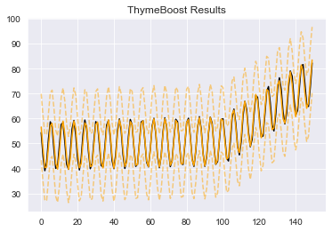
boosted_model.plot_results(output)

boosted_model.plot_components(output)

I won’t spend much time on the different parameters, just remember that fit_type='local' means that we are searching for the change points.
Overall, looks like we receive a reasonable fit. Could improve the results by increasing the number of proposal splits to try, but this visually looks ok.
Now that we see what a ‘full’ fit of the series looks like, let’s try out the new ‘update’ method- which is the online learning piece.
First, we will do our standard fit but with just 100 values:
boosted_model = tb.ThymeBoost(verbose=0,
split_strategy='gradient')
output = boosted_model.fit(y[:100],
min_sample_pct=.2,
trend_estimator=['linear'],
seasonal_estimator='fourier',
seasonal_period=25,
additive=True,
global_cost='maicc',
fit_type=['global', 'local'],
)
Next, let’s get the next batch of data to update the model with. We will call this ‘update_y’ for obvious reasons!
update_y = y[100:150]
And finally, let’s update the model with the ‘update’ method. All it takes is the output from the fit function and the updated series. Notice how I overwrite the output variable. The output of the update method is the same as the fit method:
output = boosted_model.update(output, update_y)
boosted_model.plot_results(output)
As noted, the update method allows us to use all the standard methods that fit does, such as ‘plot_results’, ‘plot_components’, and ‘predict’. Let’s see the components:
boosted_model.plot_components(output)

The results so far look good! We will usually not get identical results as a ‘full’ fit. This is due to the splits we consider when doing changepoint detection, and a few other nuances. But, the results should be comparable.
Let’s update the model again with the next 100 data points:
update_y = y[150:250]
output = boosted_model.update(output, update_y)
And finally, we will use this to predict 25 steps:
predicted_output = boosted_model.predict(output, 25)
boosted_model.plot_results(output, predicted_output)

And plotting components as before:
boosted_model.plot_components(output, predicted_output)

There we have it! A good fit from several updates and reasonable looking forecast.
Before you click away — a few important things to consider when working with this in the context of changepoints…
First off, min_sample_pct=.2 applies to the series, so if you require the model to be more reactive then decrease that value to the appropriate level such as 0.05.
Second off, not everything you pass to the fit method will work in the update method. The most important of these being multiplicative fitting and passing exogenous variable.
Lastly, actually I think those are the only considerations. At least, they are the only ones I know of! But definitely let me know if you come across any other edge cases or issues!
In this article we just covered the basic use case for online learning with ThymeBoost. The feature is still in development so if there are any issues definitely open an issue on github. As mentioned before, the feature does not allow exogenous variables or multiplicative fitting but they are on the ToDo list!
Feel free to leave a comment with any questions!
If you enjoyed this article you may enjoy a few others about ThymeBoost:
Thanks for reading!
An Example with ThymeBoost

Online learning involves updating parameters with new data without re-fitting the entire process. For models which involve boosting, such as ThymeBoost, the ability to pick up where we left off would save valuable computation time.
Luckily for us, the boosting procedure unlocks an easy path to updating parameters given new data. This is because the whole system is built to learn from residuals. Once we have new data, we simply need to predict for that new data and inject those residuals back into the procedure. The rest flows normally from there!
In this article, we will take a quick look at the new ‘update’ method for ThymeBoost which allows online learning to update the model as we receive new data.
For our example, we will generate a simple series which contains 2 trend-changepoints and some seasonality:
import numpy as np
import matplotlib.pyplot as plt
import seaborn as sns
import pandas as pd
sns.set_style('darkgrid')seasonality = ((np.cos(np.arange(1, 301))*10 + 50))
np.random.seed(100)
trend = np.linspace(-1, 1, 100)
trend = np.append(trend, np.linspace(1, 50, 100))
trend = np.append(trend, np.linspace(50, 1, 100))
y = trend + seasonality
plt.plot(y)
plt.show()
With our series in hand, let’s fit it with ThymeBoost the normal way. If you haven’t been exposed to ThymeBoost before, I recommend checking out this article which gives a good overview:
And make sure to have the most recent version from pip!
With that out of the way, let’s fit it:
from ThymeBoost import ThymeBoost as tb
boosted_model = tb.ThymeBoost(verbose=0,
n_rounds=None,
split_strategy='gradient')
output = boosted_model.fit(y,
min_sample_pct=.2,
trend_estimator=['linear'],
seasonal_estimator='fourier',
seasonal_period=25,
additive=True,
global_cost='mse',
fit_type=['local'],
)
boosted_model.plot_results(output)
boosted_model.plot_components(output)
I won’t spend much time on the different parameters, just remember that fit_type='local' means that we are searching for the change points.
Overall, looks like we receive a reasonable fit. Could improve the results by increasing the number of proposal splits to try, but this visually looks ok.
Now that we see what a ‘full’ fit of the series looks like, let’s try out the new ‘update’ method- which is the online learning piece.
First, we will do our standard fit but with just 100 values:
boosted_model = tb.ThymeBoost(verbose=0,
split_strategy='gradient')
output = boosted_model.fit(y[:100],
min_sample_pct=.2,
trend_estimator=['linear'],
seasonal_estimator='fourier',
seasonal_period=25,
additive=True,
global_cost='maicc',
fit_type=['global', 'local'],
)
Next, let’s get the next batch of data to update the model with. We will call this ‘update_y’ for obvious reasons!
update_y = y[100:150]
And finally, let’s update the model with the ‘update’ method. All it takes is the output from the fit function and the updated series. Notice how I overwrite the output variable. The output of the update method is the same as the fit method:
output = boosted_model.update(output, update_y)
boosted_model.plot_results(output)
As noted, the update method allows us to use all the standard methods that fit does, such as ‘plot_results’, ‘plot_components’, and ‘predict’. Let’s see the components:
boosted_model.plot_components(output)
The results so far look good! We will usually not get identical results as a ‘full’ fit. This is due to the splits we consider when doing changepoint detection, and a few other nuances. But, the results should be comparable.
Let’s update the model again with the next 100 data points:
update_y = y[150:250]
output = boosted_model.update(output, update_y)
And finally, we will use this to predict 25 steps:
predicted_output = boosted_model.predict(output, 25)
boosted_model.plot_results(output, predicted_output)
And plotting components as before:
boosted_model.plot_components(output, predicted_output)
There we have it! A good fit from several updates and reasonable looking forecast.
Before you click away — a few important things to consider when working with this in the context of changepoints…
First off, min_sample_pct=.2 applies to the series, so if you require the model to be more reactive then decrease that value to the appropriate level such as 0.05.
Second off, not everything you pass to the fit method will work in the update method. The most important of these being multiplicative fitting and passing exogenous variable.
Lastly, actually I think those are the only considerations. At least, they are the only ones I know of! But definitely let me know if you come across any other edge cases or issues!
In this article we just covered the basic use case for online learning with ThymeBoost. The feature is still in development so if there are any issues definitely open an issue on github. As mentioned before, the feature does not allow exogenous variables or multiplicative fitting but they are on the ToDo list!
Feel free to leave a comment with any questions!
If you enjoyed this article you may enjoy a few others about ThymeBoost:
Thanks for reading!
Denial of responsibility! Techno Blender is an automatic aggregator of the all world’s media. In each content, the hyperlink to the primary source is specified. All trademarks belong to their rightful owners, all materials to their authors. If you are the owner of the content and do not want us to publish your materials, please contact us by email – [email protected]. The content will be deleted within 24 hours.