
Optimal Transport and its Applications to Fairness
Having its roots in economics, optimal transport was developed as a tool for how to best allocate resources. The origins of the theory of optimal transport itself date back to 1781, when Gaspard Monge studied the most efficient way to move earth to build fortifications for Napoleon’s army. In its full generality, optimal transport is a problem of how to move all of the resources (e.g. iron) from a collection of origin points (iron mines) to a collection of destination points (iron factories), while minimizing the total distance the resource has to travel. Mathematically, we want to find a function that takes each origin and maps it to a destination while minimizing the total distance between the origins and their corresponding destinations. Despite its innocuous description, progress on this original formulation of the problem, called the Monge formulation, remained stalled for nearly 200 years.
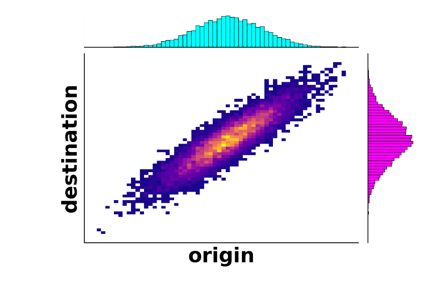
The first real leap toward a solution happened in the 1940s, when a Soviet mathematician named Leonid Kantorovich tweaked the formulation of the problem into its modern version and what is now referred to as the Monge-Kantorovich formulation. The novelty here was to allow some iron from the same mine to go to different factories. For example, 60% of the iron from a mine could go to one factory and the remaining 40% of the iron from that mine could go to a different factory. Mathematically, this is no longer a function because the same origin is now mapped to potentially many destinations. Instead, this is called a coupling between the distribution of origins and the distribution of destinations and is shown in the figure below; picking a mine from the blue distribution (origin) and traveling vertically along the figure shows the distribution of factories (destinations) where that iron was sent.
As a part of this new development, Kantorivich introduced an important concept known as the Wasserstein distance. Similar to the distance between two points on a map, the Wasserstein distance (also called the earth mover’s distance inspired by its original context) measures how far apart two distributions are, such as the blue and magenta distributions in this example. For example, if all of the iron mines are very far from all of the iron factories, then the Wasserstein distance between the distribution (locations) of mines and the distribution of factories will be very large. Even with these new improvements, it still wasn’t clear whether there actually exists a best way to transport resources, let alone what that way was. Finally, in the 1990s the theory began developing rapidly due to improvements in mathematical analysis and optimization leading to partial solutions to the problem. It was also around this time and into the 21st century that optimal transport began creeping into other fields such as particle physics, fluid dynamics, and even statistics and machine learning.
Modern Optimal Transport
With the explosion of the newly developed theory, optimal transport has found itself at the center of many new statistical and AI algorithms appearing within the last two decades. In virtually every statistical algorithm, data is modeled either explicitly or implicitly as having some underlying probability distribution. For example, if you are collecting data on an individual’s income across different countries, then there is a probability distribution for each country of that population’s income. If we want to compare two countries based on the income distributions of their populations, then we need a way to measure how far apart these two distributions are. This is exactly the reason why optimal transport, particularly the Wasserstein distance, has become so useful in data science. However, the Wasserstein distance isn’t the only measure of how far apart two probability distributions are. In fact, two alternatives — the L-2 distance and the Kullback-Leibler (KL) divergence — have been more common historically due to their connections to physics and information theory. The key advantage of the Wasserstein distance over these alternatives is that it takes both the values and their probabilities into account when computing the distance whereas the L-2 distance and KL divergence only take probabilities into account. The figure below shows an example of an artificial dataset on the income of three fictional countries.
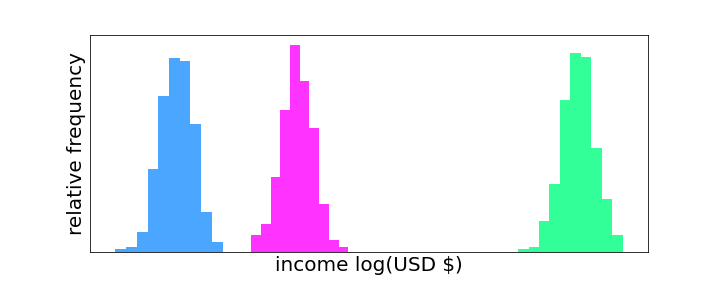
In this case, since the distributions do not overlap, the L-2 distance (or KL divergence) between the blue and magenta distributions will be roughly the same as the L-2 distance between the blue and green distributions. On the other hand, the Wasserstein distance between the blue and magenta distributions will be much smaller than the Wasserstein distance between the blue and green distributions because there is a significant difference in the values (horizontal separation). This property of the Wasserstein distance makes it well suited for quantifying differences between distributions and, in particular, datasets.
Enforcing Fairness With Optimal Transport
With massive amounts of data being collected daily and machine learning becoming more ubiquitous across many industries, data scientists have to be increasingly careful to not let their analyses and algorithms perpetuate existing biases and prejudices in the data. For example, if a dataset for home mortgage loan approvals contains information on the applicant’s ethnicity, but minorities were discriminated against during collection due to the methodology used or unconscious bias, then models trained on that data will reflect the underlying bias to some degree. Optimal transport can be leveraged to help mitigate this bias and improve fairness in two ways. The first and simplest way is to use the Wasserstein distance to identify if potential bias in the dataset exists. For example, we can estimate the Wasserstein distance between the distribution of loan amounts approved for women and the distribution of loan amounts approved for men and if the Wasserstein distance is very large, i.e. statistically significant, then we may suspect a potential bias. This idea of testing whether there is a discrepancy between two groups is known in statistics as a two-sample hypothesis test.
Alternatively, optimal transport can even be used to enforce fairness in a model when the underlying dataset itself is biased. This is extremely useful from a practical standpoint because many real datasets will exhibit some degree of bias and collecting unbiased data can be extremely costly, time-consuming, or infeasible. Therefore, it’s far more practical to use the data we have available, however imperfect it may be, and try to ensure that our model mitigates this bias. This is achieved by enforcing a constraint called Strong Demographic Parity in our model, which forces model predictions to be statistically independent of any sensitive attributes. One way to do this is to map the distribution of model predictions to a distribution of adjusted predictions that does not depend on the sensitive attributes. However, adjusting the predictions will also change the performance and accuracy of the model, and so there is a trade-off between model performance and how much the model depends on sensitive attributes, i.e., how fair it is.
Optimal transport comes into play by changing the predictions as little as possible to ensure optimal model performance while still guaranteeing that the new predictions are independent of the sensitive attributes. This new distribution of adjusted model predictions is known as the Wasserstein barycenter, which has been the subject of much research over the last decade. The Wasserstein barycenter is analogous to an average for probability distributions in the sense that it minimizes the total distance from itself to all of the other distributions. The illustration below shows three distributions (green, blue, and magenta) along with their Wasserstein barycenter in red.
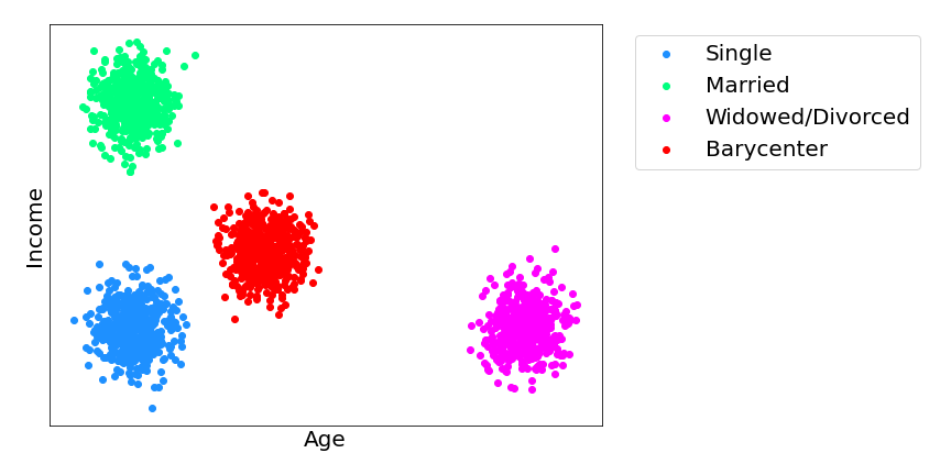
In the example above, suppose that we built a model to predict a person’s age and income based on a dataset that contains a single sensitive attribute such as marital status that can take three possible values: single (blue), married (green), and widowed/divorced (magenta). The scatter plot shows the distribution of model predictions for each of these different values. However, we want to adjust these so that the new model predictions are blind to a person’s marital status. We can use optimal transport to map each of these distributions to the barycenter in red. Because all values are mapped to the same distribution we can no longer tell a person’s marital status based on their income and age and vice versa. The barycenter preserves the model’s fidelity as much as possible.
The growing prevalence of data and machine learning models used in corporate and governmental decision-making has led to the rise of new social and ethical concerns about ensuring their fair application. Many datasets contain some sort of bias due to the nature of how they were collected, and so it is important that the models trained on them do not exacerbate this bias or any historical discrimination. Optimal transport is just one approach to tackling this problem that has been gaining momentum in recent years. Nowadays, there are fast and efficient methods for computing optimal transport maps and distances making this approach suitable for modern large datasets. Fairness has become and will remain a central issue in data science as we become more reliant on data-based models and insights and optimal transport will play a critical role in achieving this.
Having its roots in economics, optimal transport was developed as a tool for how to best allocate resources. The origins of the theory of optimal transport itself date back to 1781, when Gaspard Monge studied the most efficient way to move earth to build fortifications for Napoleon’s army. In its full generality, optimal transport is a problem of how to move all of the resources (e.g. iron) from a collection of origin points (iron mines) to a collection of destination points (iron factories), while minimizing the total distance the resource has to travel. Mathematically, we want to find a function that takes each origin and maps it to a destination while minimizing the total distance between the origins and their corresponding destinations. Despite its innocuous description, progress on this original formulation of the problem, called the Monge formulation, remained stalled for nearly 200 years.
The first real leap toward a solution happened in the 1940s, when a Soviet mathematician named Leonid Kantorovich tweaked the formulation of the problem into its modern version and what is now referred to as the Monge-Kantorovich formulation. The novelty here was to allow some iron from the same mine to go to different factories. For example, 60% of the iron from a mine could go to one factory and the remaining 40% of the iron from that mine could go to a different factory. Mathematically, this is no longer a function because the same origin is now mapped to potentially many destinations. Instead, this is called a coupling between the distribution of origins and the distribution of destinations and is shown in the figure below; picking a mine from the blue distribution (origin) and traveling vertically along the figure shows the distribution of factories (destinations) where that iron was sent.
As a part of this new development, Kantorivich introduced an important concept known as the Wasserstein distance. Similar to the distance between two points on a map, the Wasserstein distance (also called the earth mover’s distance inspired by its original context) measures how far apart two distributions are, such as the blue and magenta distributions in this example. For example, if all of the iron mines are very far from all of the iron factories, then the Wasserstein distance between the distribution (locations) of mines and the distribution of factories will be very large. Even with these new improvements, it still wasn’t clear whether there actually exists a best way to transport resources, let alone what that way was. Finally, in the 1990s the theory began developing rapidly due to improvements in mathematical analysis and optimization leading to partial solutions to the problem. It was also around this time and into the 21st century that optimal transport began creeping into other fields such as particle physics, fluid dynamics, and even statistics and machine learning.
Modern Optimal Transport
With the explosion of the newly developed theory, optimal transport has found itself at the center of many new statistical and AI algorithms appearing within the last two decades. In virtually every statistical algorithm, data is modeled either explicitly or implicitly as having some underlying probability distribution. For example, if you are collecting data on an individual’s income across different countries, then there is a probability distribution for each country of that population’s income. If we want to compare two countries based on the income distributions of their populations, then we need a way to measure how far apart these two distributions are. This is exactly the reason why optimal transport, particularly the Wasserstein distance, has become so useful in data science. However, the Wasserstein distance isn’t the only measure of how far apart two probability distributions are. In fact, two alternatives — the L-2 distance and the Kullback-Leibler (KL) divergence — have been more common historically due to their connections to physics and information theory. The key advantage of the Wasserstein distance over these alternatives is that it takes both the values and their probabilities into account when computing the distance whereas the L-2 distance and KL divergence only take probabilities into account. The figure below shows an example of an artificial dataset on the income of three fictional countries.
In this case, since the distributions do not overlap, the L-2 distance (or KL divergence) between the blue and magenta distributions will be roughly the same as the L-2 distance between the blue and green distributions. On the other hand, the Wasserstein distance between the blue and magenta distributions will be much smaller than the Wasserstein distance between the blue and green distributions because there is a significant difference in the values (horizontal separation). This property of the Wasserstein distance makes it well suited for quantifying differences between distributions and, in particular, datasets.
Enforcing Fairness With Optimal Transport
With massive amounts of data being collected daily and machine learning becoming more ubiquitous across many industries, data scientists have to be increasingly careful to not let their analyses and algorithms perpetuate existing biases and prejudices in the data. For example, if a dataset for home mortgage loan approvals contains information on the applicant’s ethnicity, but minorities were discriminated against during collection due to the methodology used or unconscious bias, then models trained on that data will reflect the underlying bias to some degree. Optimal transport can be leveraged to help mitigate this bias and improve fairness in two ways. The first and simplest way is to use the Wasserstein distance to identify if potential bias in the dataset exists. For example, we can estimate the Wasserstein distance between the distribution of loan amounts approved for women and the distribution of loan amounts approved for men and if the Wasserstein distance is very large, i.e. statistically significant, then we may suspect a potential bias. This idea of testing whether there is a discrepancy between two groups is known in statistics as a two-sample hypothesis test.
Alternatively, optimal transport can even be used to enforce fairness in a model when the underlying dataset itself is biased. This is extremely useful from a practical standpoint because many real datasets will exhibit some degree of bias and collecting unbiased data can be extremely costly, time-consuming, or infeasible. Therefore, it’s far more practical to use the data we have available, however imperfect it may be, and try to ensure that our model mitigates this bias. This is achieved by enforcing a constraint called Strong Demographic Parity in our model, which forces model predictions to be statistically independent of any sensitive attributes. One way to do this is to map the distribution of model predictions to a distribution of adjusted predictions that does not depend on the sensitive attributes. However, adjusting the predictions will also change the performance and accuracy of the model, and so there is a trade-off between model performance and how much the model depends on sensitive attributes, i.e., how fair it is.
Optimal transport comes into play by changing the predictions as little as possible to ensure optimal model performance while still guaranteeing that the new predictions are independent of the sensitive attributes. This new distribution of adjusted model predictions is known as the Wasserstein barycenter, which has been the subject of much research over the last decade. The Wasserstein barycenter is analogous to an average for probability distributions in the sense that it minimizes the total distance from itself to all of the other distributions. The illustration below shows three distributions (green, blue, and magenta) along with their Wasserstein barycenter in red.
In the example above, suppose that we built a model to predict a person’s age and income based on a dataset that contains a single sensitive attribute such as marital status that can take three possible values: single (blue), married (green), and widowed/divorced (magenta). The scatter plot shows the distribution of model predictions for each of these different values. However, we want to adjust these so that the new model predictions are blind to a person’s marital status. We can use optimal transport to map each of these distributions to the barycenter in red. Because all values are mapped to the same distribution we can no longer tell a person’s marital status based on their income and age and vice versa. The barycenter preserves the model’s fidelity as much as possible.
The growing prevalence of data and machine learning models used in corporate and governmental decision-making has led to the rise of new social and ethical concerns about ensuring their fair application. Many datasets contain some sort of bias due to the nature of how they were collected, and so it is important that the models trained on them do not exacerbate this bias or any historical discrimination. Optimal transport is just one approach to tackling this problem that has been gaining momentum in recent years. Nowadays, there are fast and efficient methods for computing optimal transport maps and distances making this approach suitable for modern large datasets. Fairness has become and will remain a central issue in data science as we become more reliant on data-based models and insights and optimal transport will play a critical role in achieving this.
Denial of responsibility! Techno Blender is an automatic aggregator of the all world’s media. In each content, the hyperlink to the primary source is specified. All trademarks belong to their rightful owners, all materials to their authors. If you are the owner of the content and do not want us to publish your materials, please contact us by email – [email protected]. The content will be deleted within 24 hours.