
Overcome the biggest obstacle in machine learning: Overfitting | by Andrew D #datascience | Aug, 2022
Overfitting is a concept in data science that occurs when a predictive model learns to generalize well on training data but not on unseen data
The best way to explain what overfitting is is through an example.
Picture this scenario: we have just been hired as a data scientist in a company that develops photo processing software. The company recently decided to implement machine learning in their processes and the intention is to create software that can distinguish original photos from edited photos.
Our task is to create a model that can detect photo edits that have human beings as subjects.
We are excited about the opportunity, and being our first job experience, we work very hard to make a good impression.
We properly train a model, which appears to perform very well on the training data. We are very happy about it, and we communicate our results to the stakeholders. The next step is to serve the model in production with a small group of users. We set up everything with the technical team and shortly after the model is online and outputs its results to the test users.
The next morning we open our inbox and read a series of discouraging messages. Users have reported very negative feedback! Our model does not seem to be able to classify images correctly. How is it possible that in the training phase our model performed well while now in production we observe such poor results?
Simple. We have been victim of overfitting.
We have lost our job. What a blow!
The example above represents a somewhat exaggerated situation. A novice analyst has at least once heard of the term overfitting. It is probably one of the first words you learn when working in the industry, following or listening to online tutorials.
Nonetheless, overfitting is a phenomenon that is practically always observed when training a predictive model. This leads the analyst to continually face the same problem which can be caused by a multitude of reasons.
In this article I will talk about what overfitting is, why it represents the biggest obstacle that an analyst faces when doing machine learning and how to prevent this from occurring through some techniques.
Although it is a fundamental concept in machine learning, explaining clearly what overfitting means is not easy. This is because you have to start from what it means to train a model and evaluate its performance. In this article I write about what machine learning is and what it implies to train a model.
Referencing from the article mentioned,
The act of showing the data to the model and allowing it to learn from it is called training.[…].During training, the model tries to learn the patterns in data based on certain assumptions. For example, probabilistic algorithms base their operations on deducing the probabilities of an event occurring in the presence of certain data.
When the model is trained, we use an evaluation metric to determine how far the model’s predictions are from the actual observed value. For example, for a classification problem (like the one in our example) we could use the F1 score to understand how the model is performing on the training data.
The mistake made by the junior analyst in the introductory example has to do with a bad interpretation of the evaluation metric during the training phase and the absence of a framework for validating the results.
In fact, the analyst paid attention to the model’s performance during training, forgetting to look at and analyze the performance on the test data.
Overfitting occurs when our model learns well to generalize training data but not test data. When this happens our algorithm fails to perform well with data it has never seen before. This completely destroys its purpose, making it a quite useless model.
This is why overfitting is an analyst’s worst enemy: it completely defeats the purpose of our work.
When a model is trained, it uses a training set to learn the patterns and map the feature set to the target variable. However, it can happen, as we have already seen, that a model can start learning noisy or even useless information — even worse, this information is only present in the training set.
Our model learns information that it does not need (or is not really present) to do its job on new, unseen data — such as those of users in a live production setting.
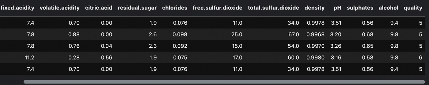
Let’s use the famous Red Wine Dataset from Kaggle to visualize a case of overfitting. This dataset has 11 dimensions that define the quality of a red wine. Based on these we have to build a model capable of predicting the quality of a red wine, which is a value between 1 and 10.
We will use a decision tree-based classifier (Sklearn.tree.DecisionTreeClassifier) to show how a model can be led to overfit.
This is what the dataset looks like if we print the first 5 lines
We use this code to train a decision tree.
Train accuracy: 0.623
Test accuracy: 0.591
We initialized our decision tree with the hyperparameter max_depth = 3. Let’s try using a different value now — for example 7.
clf = tree.DecisionTreeClassifier (max_depth = 7) # the rest of the code remains the same
Let’s look at the new values of accuracy
Train accuracy: 0.754
Test accuracy: 0.591
Accuracy is increasing for the training set, but not for the test set. We put everything in a loop where we are going to modify max_depth dynamically and training a model at each iteration.

Look how a high max_depth corresponds to a very high accuracy in training (touching values of 100%) but how this is around 55–60% in the test set.
What we are observing is overfitting!
In fact, the highest accuracy value in the test set can be seen at max_depth = 9. Above this value the accuracy does not improve. It therefore makes no sense to increase the value of the parameter above 9.
This value of max_depth = 9 represents the “sweet spot” — that is, the ideal value for not having a model that overfits, but still be able to generalize the data well.
In fact, a model could also be very “superficial” and experience underfitting, the opposite of overfitting. The “sweet spot” is in balance between these two points. The analyst’s task is to get as close as possible to this point.

The most frequent causes that lead a model to overfill are the following:
- Our data contains noise and other non-relevant information
- The training and test sets are too small
- The model is too complex
The data contains noise
When our training data contains noise, our model learns those patterns and then tries to apply that knowledge on the test set, obviously without success.
The data is little and not representative
If we have little data, those may not be sufficient to be representative of the reality that will then be provided by the users who will use the model.
The model is too complex
An overly complex model will focus on information that is fundamentally irrelevant to mapping the target variable. In the previous example, the decision tree with max_depth = 9 was neither too simple nor too complex. Increasing this value led to an increase in the performance metric in training, but not in a test setting.
There are several ways to avoid overfitting. Here we see the most common and effective ones to be used practically always
- Cross-validation
- Add more data to our dataset
- Remove features
- Use an early stopping mechanism
- Regularize the model
Each of these techniques allows the analyst to understand the performance of the model well and to reach the “sweet spot” mentioned above more quickly.
Cross-validation
Cross-validation is a very common and extremely powerful technique that allows you to test the model’s performance on several validation “mini-sets”, instead of using a single set as we have done previously. This allows us to understand how the model generalizes on different portions of the entire dataset, thus giving a clearer idea of the behavior of the model.
Add more data to our dataset
Our model can get closer to the sweet spot simply by integrating more information. We should increase the data whenever we can in order to offer our model portions of “reality” that are increasingly representative. I recommend the reader to read this article where I explain how to build a dataset from scratch.
Remove features
Feature selection techniques (such as Boruta) can help us understand which features are useless for predicting the target variable. Removing these variables can help reduce background noise observing the model.
Use an early stopping mechanism
Early stopping is a technique mainly used in deep learning and consists in stopping the model when there is no increase in performance for a series of training periods. This allows you to save the state of the model at its best time and use only this best performing version.
Regularize the model
Through the tuning of the hyperparameters we can often and willingly control the behavior of the model to reduce or increase its complexity. We can modify these hyperparameters directly during cross-validation to understand how the model performs on different data splits.
Glad you made it here. Hopefully you’ll find this article useful and implement snippets of it in your codebase.
If you want to support my content creation activity, feel free to follow my referral link below and join Medium’s membership program. I will receive a portion of your investment and you’ll be able to access Medium’s plethora of articles on data science and more in a seamless way.
Have a great day. Stay well 👋
Overfitting is a concept in data science that occurs when a predictive model learns to generalize well on training data but not on unseen data

The best way to explain what overfitting is is through an example.
Picture this scenario: we have just been hired as a data scientist in a company that develops photo processing software. The company recently decided to implement machine learning in their processes and the intention is to create software that can distinguish original photos from edited photos.
Our task is to create a model that can detect photo edits that have human beings as subjects.
We are excited about the opportunity, and being our first job experience, we work very hard to make a good impression.
We properly train a model, which appears to perform very well on the training data. We are very happy about it, and we communicate our results to the stakeholders. The next step is to serve the model in production with a small group of users. We set up everything with the technical team and shortly after the model is online and outputs its results to the test users.
The next morning we open our inbox and read a series of discouraging messages. Users have reported very negative feedback! Our model does not seem to be able to classify images correctly. How is it possible that in the training phase our model performed well while now in production we observe such poor results?
Simple. We have been victim of overfitting.
We have lost our job. What a blow!
The example above represents a somewhat exaggerated situation. A novice analyst has at least once heard of the term overfitting. It is probably one of the first words you learn when working in the industry, following or listening to online tutorials.
Nonetheless, overfitting is a phenomenon that is practically always observed when training a predictive model. This leads the analyst to continually face the same problem which can be caused by a multitude of reasons.
In this article I will talk about what overfitting is, why it represents the biggest obstacle that an analyst faces when doing machine learning and how to prevent this from occurring through some techniques.
Although it is a fundamental concept in machine learning, explaining clearly what overfitting means is not easy. This is because you have to start from what it means to train a model and evaluate its performance. In this article I write about what machine learning is and what it implies to train a model.
Referencing from the article mentioned,
The act of showing the data to the model and allowing it to learn from it is called training.[…].During training, the model tries to learn the patterns in data based on certain assumptions. For example, probabilistic algorithms base their operations on deducing the probabilities of an event occurring in the presence of certain data.
When the model is trained, we use an evaluation metric to determine how far the model’s predictions are from the actual observed value. For example, for a classification problem (like the one in our example) we could use the F1 score to understand how the model is performing on the training data.
The mistake made by the junior analyst in the introductory example has to do with a bad interpretation of the evaluation metric during the training phase and the absence of a framework for validating the results.
In fact, the analyst paid attention to the model’s performance during training, forgetting to look at and analyze the performance on the test data.
Overfitting occurs when our model learns well to generalize training data but not test data. When this happens our algorithm fails to perform well with data it has never seen before. This completely destroys its purpose, making it a quite useless model.
This is why overfitting is an analyst’s worst enemy: it completely defeats the purpose of our work.
When a model is trained, it uses a training set to learn the patterns and map the feature set to the target variable. However, it can happen, as we have already seen, that a model can start learning noisy or even useless information — even worse, this information is only present in the training set.
Our model learns information that it does not need (or is not really present) to do its job on new, unseen data — such as those of users in a live production setting.
Let’s use the famous Red Wine Dataset from Kaggle to visualize a case of overfitting. This dataset has 11 dimensions that define the quality of a red wine. Based on these we have to build a model capable of predicting the quality of a red wine, which is a value between 1 and 10.
We will use a decision tree-based classifier (Sklearn.tree.DecisionTreeClassifier) to show how a model can be led to overfit.
This is what the dataset looks like if we print the first 5 lines
We use this code to train a decision tree.
Train accuracy: 0.623
Test accuracy: 0.591
We initialized our decision tree with the hyperparameter max_depth = 3. Let’s try using a different value now — for example 7.
clf = tree.DecisionTreeClassifier (max_depth = 7) # the rest of the code remains the same
Let’s look at the new values of accuracy
Train accuracy: 0.754
Test accuracy: 0.591
Accuracy is increasing for the training set, but not for the test set. We put everything in a loop where we are going to modify max_depth dynamically and training a model at each iteration.
Look how a high max_depth corresponds to a very high accuracy in training (touching values of 100%) but how this is around 55–60% in the test set.
What we are observing is overfitting!
In fact, the highest accuracy value in the test set can be seen at max_depth = 9. Above this value the accuracy does not improve. It therefore makes no sense to increase the value of the parameter above 9.
This value of max_depth = 9 represents the “sweet spot” — that is, the ideal value for not having a model that overfits, but still be able to generalize the data well.
In fact, a model could also be very “superficial” and experience underfitting, the opposite of overfitting. The “sweet spot” is in balance between these two points. The analyst’s task is to get as close as possible to this point.
The most frequent causes that lead a model to overfill are the following:
- Our data contains noise and other non-relevant information
- The training and test sets are too small
- The model is too complex
The data contains noise
When our training data contains noise, our model learns those patterns and then tries to apply that knowledge on the test set, obviously without success.
The data is little and not representative
If we have little data, those may not be sufficient to be representative of the reality that will then be provided by the users who will use the model.
The model is too complex
An overly complex model will focus on information that is fundamentally irrelevant to mapping the target variable. In the previous example, the decision tree with max_depth = 9 was neither too simple nor too complex. Increasing this value led to an increase in the performance metric in training, but not in a test setting.
There are several ways to avoid overfitting. Here we see the most common and effective ones to be used practically always
- Cross-validation
- Add more data to our dataset
- Remove features
- Use an early stopping mechanism
- Regularize the model
Each of these techniques allows the analyst to understand the performance of the model well and to reach the “sweet spot” mentioned above more quickly.
Cross-validation
Cross-validation is a very common and extremely powerful technique that allows you to test the model’s performance on several validation “mini-sets”, instead of using a single set as we have done previously. This allows us to understand how the model generalizes on different portions of the entire dataset, thus giving a clearer idea of the behavior of the model.
Add more data to our dataset
Our model can get closer to the sweet spot simply by integrating more information. We should increase the data whenever we can in order to offer our model portions of “reality” that are increasingly representative. I recommend the reader to read this article where I explain how to build a dataset from scratch.
Remove features
Feature selection techniques (such as Boruta) can help us understand which features are useless for predicting the target variable. Removing these variables can help reduce background noise observing the model.
Use an early stopping mechanism
Early stopping is a technique mainly used in deep learning and consists in stopping the model when there is no increase in performance for a series of training periods. This allows you to save the state of the model at its best time and use only this best performing version.
Regularize the model
Through the tuning of the hyperparameters we can often and willingly control the behavior of the model to reduce or increase its complexity. We can modify these hyperparameters directly during cross-validation to understand how the model performs on different data splits.
Glad you made it here. Hopefully you’ll find this article useful and implement snippets of it in your codebase.
If you want to support my content creation activity, feel free to follow my referral link below and join Medium’s membership program. I will receive a portion of your investment and you’ll be able to access Medium’s plethora of articles on data science and more in a seamless way.
Have a great day. Stay well 👋
Denial of responsibility! Techno Blender is an automatic aggregator of the all world’s media. In each content, the hyperlink to the primary source is specified. All trademarks belong to their rightful owners, all materials to their authors. If you are the owner of the content and do not want us to publish your materials, please contact us by email – [email protected]. The content will be deleted within 24 hours.