
Particle Swarm Optimization (PSO) from scratch. Simplest explanation in python
How to implement PSO
Before talking about swarms and particles, let’s briefly discuss optimization itself. Basically, optimization is the process of finding the minima or maxima of some function. For instance, when you need to get to your office ASAP and think about which way is the fastest, you’re optimizing your route (in this case it’s a function). In math, there are literally hundreds of ways of optimization, and among them a sub-group called nature-inspired exists.
Nature-inspired algorithms are based on phenomena which draw inspiration from natural phenomena or processes. Among the most popular ones are Genetic Algorithm, Cuckoo Search, Ant Colony and Particle Swarm Optimization [1] or PSO.
This tutorial is implemented in python using only numpy and matplotlib. To follow up you can use this notebook.
Let’s start with creating a function which we’ll be optimizing using PSO.
If someone asks me to think about functions, the first thing that comes to my mind (it almost reflexive😂) is parabola. So let’s plot it firstly.
import numpy as np
import numpy.random as rnd
import matplotlib.pyplot as plt

x = np.arange(-10,10, 0.01)
y = x**2
plt.plot(x,y, lw=3)
plt.xlabel('x')
plt.ylabel('y')
plt.grid(True)
plt.show()
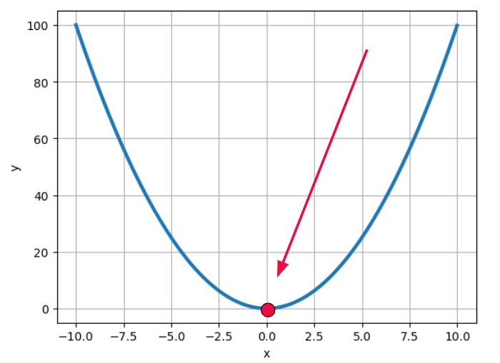
In case of this function, y=x², the goal of optimization is to find the point x=0, so y has the lowest value possible — 0. But it’s too easy. Let’s overcomplicate everything, but stay in 2D space. I decided to use the following system of equations:

Or in code:
def function(x):
  y = []
  for i in x:
    if i>-3:
      y.append(i**2-4*i+i**3)
    else:
      y.append(0.2*i**2)
  return y
x = np.arange(-10,3, 0.001)
y = function(x)
plt.plot(x,y, lw=3)
plt.title('Function to optimize')
plt.xlabel('x')
plt.ylabel('y')
plt.grid(True)
plt.show()

As you can see I intentionally made two minima: global (left) and local (right). Often when optimizing a function, we need to find the lowest (greatest) value possible, i.e. global minimum (maximum), so I wanted the PSO algorithm to face the challenge of two extrema.
Now let’s discuss the algorithm itself.
The underlying idea is based on two terms: population and swarm. Swarm consists of populations which comprise particles.
particle — — — > population — — → swarm
What is a particle in this case then? A particle is a possible solution. Imagine that you’re investigating a crime and a bunch of suspects are standing in front of you. All of them are “candidates” to be convicted. But in the case of particles, the candidates are cooperating and have social influence.
The particles themselves has two features — position and velocity (or speed; our particles are flying, right?). So these particles iteratively, one step at a time, change their positions. Their velocity is defined by the following formula:

As you can see, there are three components. The first is inertia. This is the velocity of the particle from the previous iteration multiplied by an arbitrary weight w. So it basically defines how much the previous speed of the particle affects the current one.
The second one is personal influence. It has its own coefficients: an arbitrary weight c₁ and random number r₁. In the brackets we have a difference between the best position of a particle in a population and the position of the current particle (p).
The third part is social influence. It has similar arbitrary weight c₂ and random number r₂, as well as the difference between the best position of a particle in a swarm and the position of the current particle (p).
After calculating the velocity we update the current positions of the particle simply by summation:

By now there is one big question left: what are these best position in the swarm and population?
To calculate them we need a gain/reward function indicating which solution is closer to the minimum (maximum). In our example, this gain function is the function we plotted. So the particles are Xs, and by substituting each X to the function, we can figure out which X gives the lowest (greatest) value of Y.
Thus, the best position in a population is X, which gives the lowest (greatest) Y on the current iteration. And the best position in a swarm is X which gives the lowest (greatest) Y across all the previous iterations.
So simplifying everything, we can say that the idea of the algorithm is the following:
A bunch of particles, each having a certain position and velocity, are flying together in a search of the global minimum (maximum), forming a population. Populations appear iteratively and live during only one iteration, but they exchange information with each other, so each following population is closer to finding the solution than the previous one.
Now let’s get back to coding and implement in python what we’ve discussed.
First of all, let’s define our hypoparameters. Like in many other metaheuristic algorithms, these variables should be adjusted on the way, and there is no versatile set of values. But let’s stick to these ones:
POP_SIZE = 10 #population size
MAX_ITER = 30 #the amount of optimization iterations
w = 0.2 #inertia weight
c1 = 1 #personal acceleration factor
c2 = 2 #social acceleration factor
Now let’s create a function which would generate a random population:
def populate(size):
  x1,x2 = -10, 3 #x1, x2 = right and left boundaries of our X axis
  pop = rnd.uniform(x1,x2, size) # size = amount of particles in population
  return pop
If we visualize it, we’ll get something like this:
x1=populate(50)
y1=function(x1)

plt.plot(x,y, lw=3, label='Func to optimize')
plt.plot(x1,y1,marker='o', ls='', label='Particles')
plt.xlabel('x')
plt.ylabel('y')
plt.legend()
plt.grid(True)
plt.show()

Here you can see that I randomly initialized a population of 50 particles, some of which are already close to the solution.
Now let’s implement the PSO algorithm itself. I commented each row in the code, but if you have any questions, feel free to ask in the comments below.
"""Particle Swarm Optimization (PSO)"""
particles = populate(POP_SIZE) #generating a set of particles
velocities = np.zeros(np.shape(particles)) #velocities of the particles
gains = -np.array(function(particles)) #calculating function values for the population

best_positions = np.copy(particles) #it's our first iteration, so all positions are the best
swarm_best_position = particles[np.argmax(gains)] #x with with the highest gain
swarm_best_gain = np.max(gains) #highest gain

l = np.empty((MAX_ITER, POP_SIZE)) #array to collect all pops to visualize afterwards

for i in range(MAX_ITER):

    l[i] = np.array(np.copy(particles)) #collecting a pop to visualize

    r1 = rnd.uniform(0, 1, POP_SIZE) #defining a random coefficient for personal behavior
    r2 = rnd.uniform(0, 1, POP_SIZE) #defining a random coefficient for social behavior

    velocities = np.array(w * velocities + c1 * r1 * (best_positions - particles) + c2 * r2 * (swarm_best_position - particles)) #calculating velocities

    particles+=velocities #updating position by adding the velocity

    new_gains = -np.array(function(particles)) #calculating new gains

    idx = np.where(new_gains > gains) #getting index of Xs, which have a greater gain now
    best_positions[idx] = particles[idx] #updating the best positions with the new particles
    gains[idx] = new_gains[idx] #updating gains

    if np.max(new_gains) > swarm_best_gain: #if current maxima is greateer than across all previous iters, than assign
        swarm_best_position = particles[np.argmax(new_gains)] #assigning the best candidate solution
        swarm_best_gain = np.max(new_gains) #assigning the best gain

    print(f'Iteration {i+1} \tGain: {swarm_best_gain}')
After 30 iteration we’ve got this:

As you can see the algorithm fell into the local minimum, which is not what we wanted. That’s why we need to tune our hypoparameters and start again. This time I decided to set inertia weight w=0.8, thus, now the previous velocity has a greater impact on the current state.

And voila, we reached the global minimum of the function. I strongly encourage you to play around with POP_SIZE, c₁ and c₂. It’ll allow you to gain a better understanding of the code and the idea behind PSO. If you’re interested you can complicate the task and optimize some 3D function and make a nice visualization.
===========================================
[1]Shi Y. Particle swarm optimization //IEEE connections. — 2004. — Т. 2. — №. 1. — С. 8–13.
===========================================
All my articles on Medium are free and open-access, that’s why I’d really appreciate if you followed me here!
P.s. I’m extremely passionate about (Geo)Data Science, ML/AI and Climate Change. So if you want to work together on some project pls contact me in LinkedIn.
🛰️Follow for more🛰️
Particle Swarm Optimization (PSO) from scratch. Simplest explanation in python was originally published in Towards Data Science on Medium, where people are continuing the conversation by highlighting and responding to this story.
How to implement PSO

Before talking about swarms and particles, let’s briefly discuss optimization itself. Basically, optimization is the process of finding the minima or maxima of some function. For instance, when you need to get to your office ASAP and think about which way is the fastest, you’re optimizing your route (in this case it’s a function). In math, there are literally hundreds of ways of optimization, and among them a sub-group called nature-inspired exists.
Nature-inspired algorithms are based on phenomena which draw inspiration from natural phenomena or processes. Among the most popular ones are Genetic Algorithm, Cuckoo Search, Ant Colony and Particle Swarm Optimization [1] or PSO.
This tutorial is implemented in python using only numpy and matplotlib. To follow up you can use this notebook.
Let’s start with creating a function which we’ll be optimizing using PSO.
If someone asks me to think about functions, the first thing that comes to my mind (it almost reflexive😂) is parabola. So let’s plot it firstly.
import numpy as np
import numpy.random as rnd
import matplotlib.pyplot as plt

x = np.arange(-10,10, 0.01)
y = x**2
plt.plot(x,y, lw=3)
plt.xlabel('x')
plt.ylabel('y')
plt.grid(True)
plt.show()
In case of this function, y=x², the goal of optimization is to find the point x=0, so y has the lowest value possible — 0. But it’s too easy. Let’s overcomplicate everything, but stay in 2D space. I decided to use the following system of equations:
Or in code:
def function(x):
  y = []
  for i in x:
    if i>-3:
      y.append(i**2-4*i+i**3)
    else:
      y.append(0.2*i**2)
  return y
x = np.arange(-10,3, 0.001)
y = function(x)
plt.plot(x,y, lw=3)
plt.title('Function to optimize')
plt.xlabel('x')
plt.ylabel('y')
plt.grid(True)
plt.show()
As you can see I intentionally made two minima: global (left) and local (right). Often when optimizing a function, we need to find the lowest (greatest) value possible, i.e. global minimum (maximum), so I wanted the PSO algorithm to face the challenge of two extrema.
Now let’s discuss the algorithm itself.
The underlying idea is based on two terms: population and swarm. Swarm consists of populations which comprise particles.
particle — — — > population — — → swarm
What is a particle in this case then? A particle is a possible solution. Imagine that you’re investigating a crime and a bunch of suspects are standing in front of you. All of them are “candidates” to be convicted. But in the case of particles, the candidates are cooperating and have social influence.
The particles themselves has two features — position and velocity (or speed; our particles are flying, right?). So these particles iteratively, one step at a time, change their positions. Their velocity is defined by the following formula:
As you can see, there are three components. The first is inertia. This is the velocity of the particle from the previous iteration multiplied by an arbitrary weight w. So it basically defines how much the previous speed of the particle affects the current one.
The second one is personal influence. It has its own coefficients: an arbitrary weight c₁ and random number r₁. In the brackets we have a difference between the best position of a particle in a population and the position of the current particle (p).
The third part is social influence. It has similar arbitrary weight c₂ and random number r₂, as well as the difference between the best position of a particle in a swarm and the position of the current particle (p).
After calculating the velocity we update the current positions of the particle simply by summation:
By now there is one big question left: what are these best position in the swarm and population?
To calculate them we need a gain/reward function indicating which solution is closer to the minimum (maximum). In our example, this gain function is the function we plotted. So the particles are Xs, and by substituting each X to the function, we can figure out which X gives the lowest (greatest) value of Y.
Thus, the best position in a population is X, which gives the lowest (greatest) Y on the current iteration. And the best position in a swarm is X which gives the lowest (greatest) Y across all the previous iterations.
So simplifying everything, we can say that the idea of the algorithm is the following:
A bunch of particles, each having a certain position and velocity, are flying together in a search of the global minimum (maximum), forming a population. Populations appear iteratively and live during only one iteration, but they exchange information with each other, so each following population is closer to finding the solution than the previous one.
Now let’s get back to coding and implement in python what we’ve discussed.
First of all, let’s define our hypoparameters. Like in many other metaheuristic algorithms, these variables should be adjusted on the way, and there is no versatile set of values. But let’s stick to these ones:
POP_SIZE = 10 #population size
MAX_ITER = 30 #the amount of optimization iterations
w = 0.2 #inertia weight
c1 = 1 #personal acceleration factor
c2 = 2 #social acceleration factor
Now let’s create a function which would generate a random population:
def populate(size):
  x1,x2 = -10, 3 #x1, x2 = right and left boundaries of our X axis
  pop = rnd.uniform(x1,x2, size) # size = amount of particles in population
  return pop
If we visualize it, we’ll get something like this:
x1=populate(50)
y1=function(x1)

plt.plot(x,y, lw=3, label='Func to optimize')
plt.plot(x1,y1,marker='o', ls='', label='Particles')
plt.xlabel('x')
plt.ylabel('y')
plt.legend()
plt.grid(True)
plt.show()
Here you can see that I randomly initialized a population of 50 particles, some of which are already close to the solution.
Now let’s implement the PSO algorithm itself. I commented each row in the code, but if you have any questions, feel free to ask in the comments below.
"""Particle Swarm Optimization (PSO)"""
particles = populate(POP_SIZE) #generating a set of particles
velocities = np.zeros(np.shape(particles)) #velocities of the particles
gains = -np.array(function(particles)) #calculating function values for the population

best_positions = np.copy(particles) #it's our first iteration, so all positions are the best
swarm_best_position = particles[np.argmax(gains)] #x with with the highest gain
swarm_best_gain = np.max(gains) #highest gain

l = np.empty((MAX_ITER, POP_SIZE)) #array to collect all pops to visualize afterwards

for i in range(MAX_ITER):

    l[i] = np.array(np.copy(particles)) #collecting a pop to visualize

    r1 = rnd.uniform(0, 1, POP_SIZE) #defining a random coefficient for personal behavior
    r2 = rnd.uniform(0, 1, POP_SIZE) #defining a random coefficient for social behavior

    velocities = np.array(w * velocities + c1 * r1 * (best_positions - particles) + c2 * r2 * (swarm_best_position - particles)) #calculating velocities

    particles+=velocities #updating position by adding the velocity

    new_gains = -np.array(function(particles)) #calculating new gains

    idx = np.where(new_gains > gains) #getting index of Xs, which have a greater gain now
    best_positions[idx] = particles[idx] #updating the best positions with the new particles
    gains[idx] = new_gains[idx] #updating gains

    if np.max(new_gains) > swarm_best_gain: #if current maxima is greateer than across all previous iters, than assign
        swarm_best_position = particles[np.argmax(new_gains)] #assigning the best candidate solution
        swarm_best_gain = np.max(new_gains) #assigning the best gain

    print(f'Iteration {i+1} \tGain: {swarm_best_gain}')
After 30 iteration we’ve got this:
As you can see the algorithm fell into the local minimum, which is not what we wanted. That’s why we need to tune our hypoparameters and start again. This time I decided to set inertia weight w=0.8, thus, now the previous velocity has a greater impact on the current state.
And voila, we reached the global minimum of the function. I strongly encourage you to play around with POP_SIZE, c₁ and c₂. It’ll allow you to gain a better understanding of the code and the idea behind PSO. If you’re interested you can complicate the task and optimize some 3D function and make a nice visualization.
===========================================
[1]Shi Y. Particle swarm optimization //IEEE connections. — 2004. — Т. 2. — №. 1. — С. 8–13.
===========================================
All my articles on Medium are free and open-access, that’s why I’d really appreciate if you followed me here!
P.s. I’m extremely passionate about (Geo)Data Science, ML/AI and Climate Change. So if you want to work together on some project pls contact me in LinkedIn.
🛰️Follow for more🛰️
Particle Swarm Optimization (PSO) from scratch. Simplest explanation in python was originally published in Towards Data Science on Medium, where people are continuing the conversation by highlighting and responding to this story.
Denial of responsibility! Techno Blender is an automatic aggregator of the all world’s media. In each content, the hyperlink to the primary source is specified. All trademarks belong to their rightful owners, all materials to their authors. If you are the owner of the content and do not want us to publish your materials, please contact us by email – [email protected]. The content will be deleted within 24 hours.