
Prediction Intervals in Python. Learn three ways to obtain prediction… | by Zolzaya Luvsandorj | Aug, 2022
Data Science Fundamentals
Learn three ways to obtain prediction intervals
If I ask you to guess how many movies I watched in the past week, would you feel more confident to guess “2 to 6” or “3”? We would probably agree that guessing with a range gives us a better chance of being correct than guessing with a single number. Similarly, a prediction interval gives us a more reliable and transparent estimate than a single-value prediction. In this post, we will learn three ways to obtain prediction intervals in Python.
We will start by loading necessary libraries and sample data. We will use Scikit-learn’s built-in dataset on diabetes (the data is available under BSD Licence). If you want to learn more about the dataset, check out its description with print(diabetes[‘DESCR’]).
import numpy as np
np.set_printoptions(
formatter={'float': lambda x: "{:.4f}".format(x)}
)
import pandas as pd
pd.options.display.float_format = "{:.4f}".format
from scipy.stats import t
import statsmodels.api as sm
from sklearn.datasets import load_diabetes
from sklearn.model_selection import train_test_split
from sklearn.linear_model import LinearRegression
from sklearn.ensemble import GradientBoostingRegressorimport matplotlib.pyplot as plt
import seaborn as sns
sns.set(style='darkgrid', context='talk')diabetes = load_diabetes(as_frame=True)
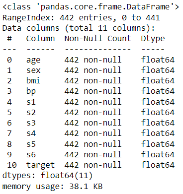
df = diabetes['data']
df['target'] = diabetes['target']
df.info()
Let’s partition the data into training and test sets:
train, test = train_test_split(df, test_size=0.1, random_state=42)
X_train, X_test, y_train, y_test = train_test_split(
df.drop(columns='target'), df['target'], test_size=0.1,
random_state=42
)
x_train = X_train['bmi']
x_test = X_test['bmi']print(f"X_train shape: {X_train.shape}")
print(f"x_train shape: {x_train.shape}")
print(f"y_train shape: {y_train.shape}")
print("\n========== Training data ==========")
display(train[['target']].describe().T)print(f"X_test shape: {X_test.shape}")
print(f"x_test shape: {x_test.shape}")
print(f"y_test shape: {y_test.shape}")print("\n========== Test data ==========")
test[['target']].describe().T
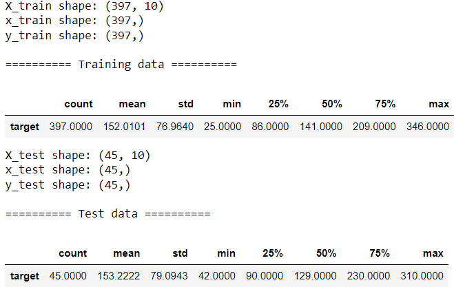
The target ranges from 25 to 350 with mean of approximately 150 and median around 130–140.
We will now look at three approaches to obtain prediction interval.
💡 1.1. Using standard errors
Let’s build a simple linear regression using bmi to predict the target.
model = LinearRegression()
model.fit(x_train.values.reshape(-1, 1), y_train)
print(f"Intercept: {model.intercept_:.2f}")
print(f"Slope: {model.coef_[0]:.2f}")
print(model.predict(x_test.values.reshape(-1, 1))[:5])
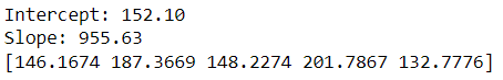
We can see the predictions, our best guess. Using the formula below, we can calculate the standard error and obtain prediction intervals:
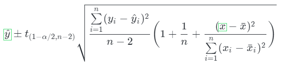
The formula can be translated into code as follows. We are using a custom object as it allows more flexibility than a function:
class CustomLinearRegression:
def __init__(self):
passdef fit(self, x, y):
# Calculate stats
self.n = len(x)
self.x_mean = np.mean(x)
self.y_mean = np.mean(y)
self.x_gap = x-self.x_mean
self.y_gap = y-self.y_mean
self.ss = np.square(self.x_gap).sum()
# Find coefficients
self.slope = np.dot(self.x_gap, self.y_gap)/self.ss
self.intercept = self.y_mean-self.slope*self.x_mean
# Find training error
y_pred = self.intercept+self.slope*x
self.se_regression = np.sqrt(
np.square(y-y_pred).sum()/(self.n-2)
)
def predict(self, x):
y_pred = self.intercept+self.slope*x
return y_pred
def predict_interval(self, x, alpha=0.1):
t_stat = t.ppf(1-alpha/2, df=self.n-2)
# Calculate interval upper and lower boundaries
df = pd.DataFrame({'x': x})
for i, value in df['x'].iteritems():
se = self.se_regression * np.sqrt(
1+1/self.n+np.square(value-self.x_mean)/self.ss
)
df.loc[i, 'y_pred'] = self.intercept+self.slope*value
df.loc[i, 'lower'] = df.loc[i, 'y_pred']-t_stat*se
df.loc[i, 'upper'] = df.loc[i, 'y_pred']+t_stat*se
return df
custom_model = CustomLinearRegression()
custom_model.fit(x_train, y_train)
print(f"Intercept: {custom_model.intercept:.2f}")
print(f"Slope: {custom_model.slope:.2f}")
custom_pred = custom_model.predict_interval(x_test)
custom_pred.head()
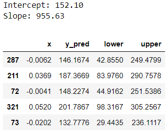
Let’s understand this output. In linear regression, predictions represent conditional mean target value. So y_pred, our prediction column, tells us the estimated mean target given the features. Prediction intervals tell us a range of values the target can take for a given record. We can see the lower and upper boundary of the prediction interval from lower and upper columns. This is a 90% prediction interval because we chose alpha=0.1. We will be using the same alpha value for the remainder of this post.
If you are curious, here’re a few ways to interpret prediction intervals:
- There is 90% probability that the actual target value for record 287 will be between 42.8550 and 249.4799.
- We are 90% confident that the actual target value for for record 287 will fall somewhere between 42.8550 and 249.4799 based on their
bmivalue. - Approximately 90% of prediction intervals will contain the actual value.
Let’s examine what percentage of target values in the test data were within the prediction intervals:
custom_correct = np.mean(
(custom_pred['lower']<y_test) & (y_test<custom_pred['upper'])
)
print(f"{custom_correct:.2%} of the prediction intervals contain true target.")

This is roughly 90%. While calculating manually helps us understand what is happening under the hood, more practically, we can use libraries and simplify our work. Here’s how we can use statsmodels package to get the same prediction interval:
sm_model = sm.OLS(y_train, sm.add_constant(x_train)).fit()
print(f"Intercept: {sm_model.params[0]:.2f}")
print(f"Slope: {sm_model.params[1]:.2f}")sm_pred = sm_model.get_prediction(sm.add_constant(x_test))\
.summary_frame(alpha=0.1)
sm_pred.head()
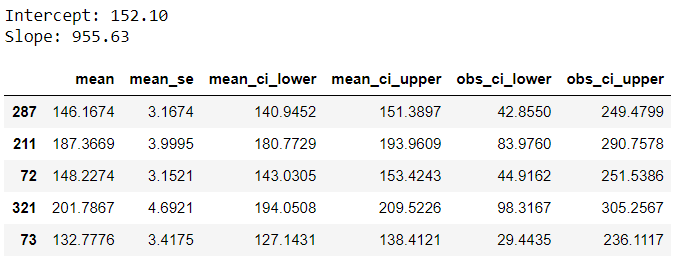
This output provides some additional outputs, let’s understand the key ones:
◼️ mean: Prediction, same as y_pred from earlier.
◼️ mean_ci_lower & mean_ci_upper: Confidence interval boundaries
◼️ obs_ci_lower & obs_ci_upper: Prediction interval boundaries, same as lower and upper from earlier.
We can check if predictions and prediction intervals match with manually calculated ones:
np.mean(np.isclose(
custom_pred.drop(columns='x').values,
sm_pred[['mean', 'obs_ci_lower', 'obs_ci_upper']]),
axis=0)
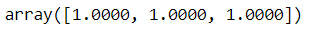
Lovely, it matches!
Now, you may be wondering what the differences between confidence and predictions intervals are. Although these terms are related and sound somewhat similar, they refer to two different intervals and shouldn’t be used interchangeably:
◼️ Confidence intervals are for mean predictions. Unlike prediction interval, confidence interval doesn’t tell us a range of target values an observation can take. Instead, it tells us a range of target mean values. Here’s an example interpretation: There is 90% probability that mean target value for records with feature values same as record 287 will fall somewhere between 140.9452 and 151.3897.
◼️ While both intervals are centred around the prediction, the standard errors for prediction intervals is bigger than the one for confidence intervals. As a result, prediction intervals are wider than confidence intervals.
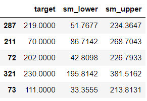
We looked at simple linear regression to get started with the concept, but it’s more common to have multiple features in practice. It’s time to expand our example to use the full set of features:
ols = sm.OLS(y_train, sm.add_constant(X_train)).fit()
test[['ols_lower', 'ols_upper']] = (ols
.get_prediction(sm.add_constant(X_test))
.summary_frame(alpha=0.1)[['obs_ci_lower', 'obs_ci_upper']])
columns = ['target', 'ols_lower', 'ols_upper']
test.head()
The flow is exactly the same as using a single feature. If you are curious to know how the formula changes in the presence of multiple features, check out this guide. Let’s evaluate our intervals:
ols_correct = np.mean(
test['target'].between(test['ols_lower'], test['ols_upper'])
)
print(f"{ols_correct:.2%} of the prediction intervals contain true target.")

1.2. From quantile regression
Using quantile regression, we can predict conditional quantile of the target instead of conditional mean target. To get 90% prediction interval, we will build two quantile regressions, one to predict 5th percentile and another to predict 95th percentile.
alpha = 0.1
quant_lower = sm.QuantReg(
y_train, sm.add_constant(X_train)
).fit(q=alpha/2)
test['quant_lower'] = quant_lower.predict(
sm.add_constant(X_test)
)quant_upper = sm.QuantReg(
y_train, sm.add_constant(X_train)
).fit(q=1-alpha/2)
test['quant_upper'] = quant_upper.predict(
sm.add_constant(X_test)
)
columns.extend(['quant_lower', 'quant_upper'])
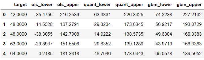
test.head()
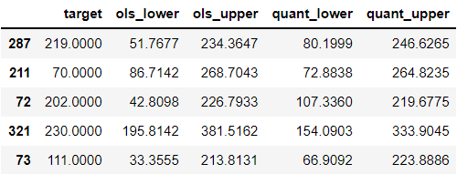
Here, quant_lower model underpredicts whereas quant_upper model overpredicts. Let’s now check the percentage of the predictions that were within the new intervals:
quant_correct = np.mean(
test['target'].between(test['quant_lower'], test['quant_upper'])
)
print(f"{quant_correct:.2%} of the prediction intervals contain true target.")

Just under 90%, slightly lower coverage than before.
1.3. From GBM with quantile loss
This last approach is very similar to the previous approach. We will use GradientBoostingRegressor with quantile loss to get 90% prediction interval using two models:
gbm_lower = GradientBoostingRegressor(
loss="quantile", alpha=alpha/2, random_state=0
)
gbm_upper = GradientBoostingRegressor(
loss="quantile", alpha=1-alpha/2, random_state=0
)gbm_lower.fit(X_train, y_train)
gbm_upper.fit(X_train, y_train)test['gbm_lower'] = gbm_lower.predict(X_test)
test['gbm_upper'] = gbm_upper.predict(X_test)
columns.extend(['gbm_lower', 'gbm_upper'])
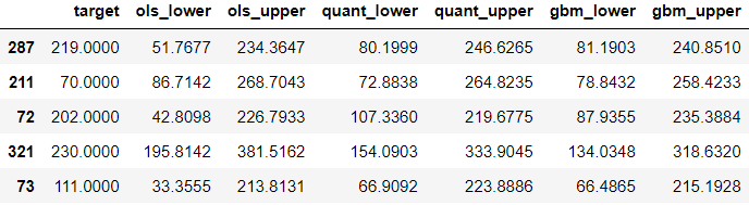
test.head()
Time to evaluate the coverage of the interval:
gbm_correct = np.mean(
test['target'].between(test['gbm_lower'], test['gbm_upper'])
)
print(f"{gbm_correct:.2%} of the prediction intervals contain true target.")

This is lower compared to the previous intervals. Looking at the sample records above, the intervals look slightly more narrow compared to the previous two approaches. For any of the approaches we learned in this post, we can increase this coverage percentage by reducing alpha. However, this means that the intervals can become too wide to the point that they may be less informative or helpful in decision making. So we must thrive to find the right balance when using prediction intervals.
Let’s now compare all three intervals visually:
test = test.sort_values('target').reset_index()plt.figure(figsize=(10,6))
sns.scatterplot(data=test, x=test.index, y='target',
color='grey')
sns.lineplot(data=test, x=test.index, y='ols_lower',
color='hotpink')
sns.lineplot(data=test, x=test.index, y='ols_upper',
color='hotpink', label='Linear Regression')sns.lineplot(data=test, x=test.index, y='quant_lower',
color='blue')
sns.lineplot(data=test, x=test.index, y='quant_upper',
color='blue', label='Quantile Regression')sns.lineplot(data=test, x=test.index, y='gbm_lower',
color='green')
sns.lineplot(data=test, x=test.index, y='gbm_upper',
color='green', label='Gradient Boosting Machine')
plt.xticks([]);
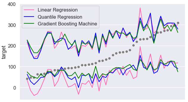
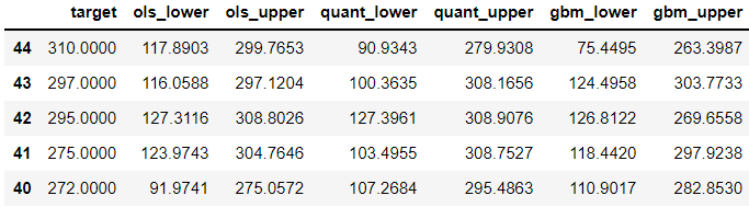
Values closer to the min and max appear to be more likely to be outside the prediction intervals. Let’s look further into these errors. We will look at 5 records with the highest target:
test.nlargest(5, 'target')
Now, let’s look at the other end:
test.nsmallest(5, 'target')
The lower boundary of the linear regression prediction interval is sometimes negative. This is something to be mindful of. If we know the target is going to be always positive, we can overwrite these negative boundaries with the lowest possible value using a wrapper function.
Voila, these were the three ways to calculate prediction interval! Hope you get to use these approach in your next regression use-case.
Would you like to access more content like this? Medium members get unlimited access to any articles on Medium. If you become a member using my referral link, a portion of your membership fee will directly go to support me.
Data Science Fundamentals
Learn three ways to obtain prediction intervals
If I ask you to guess how many movies I watched in the past week, would you feel more confident to guess “2 to 6” or “3”? We would probably agree that guessing with a range gives us a better chance of being correct than guessing with a single number. Similarly, a prediction interval gives us a more reliable and transparent estimate than a single-value prediction. In this post, we will learn three ways to obtain prediction intervals in Python.
We will start by loading necessary libraries and sample data. We will use Scikit-learn’s built-in dataset on diabetes (the data is available under BSD Licence). If you want to learn more about the dataset, check out its description with print(diabetes[‘DESCR’]).
import numpy as np
np.set_printoptions(
formatter={'float': lambda x: "{:.4f}".format(x)}
)
import pandas as pd
pd.options.display.float_format = "{:.4f}".format
from scipy.stats import t
import statsmodels.api as sm
from sklearn.datasets import load_diabetes
from sklearn.model_selection import train_test_split
from sklearn.linear_model import LinearRegression
from sklearn.ensemble import GradientBoostingRegressorimport matplotlib.pyplot as plt
import seaborn as sns
sns.set(style='darkgrid', context='talk')diabetes = load_diabetes(as_frame=True)
df = diabetes['data']
df['target'] = diabetes['target']
df.info()
Let’s partition the data into training and test sets:
train, test = train_test_split(df, test_size=0.1, random_state=42)
X_train, X_test, y_train, y_test = train_test_split(
df.drop(columns='target'), df['target'], test_size=0.1,
random_state=42
)
x_train = X_train['bmi']
x_test = X_test['bmi']print(f"X_train shape: {X_train.shape}")
print(f"x_train shape: {x_train.shape}")
print(f"y_train shape: {y_train.shape}")
print("\n========== Training data ==========")
display(train[['target']].describe().T)print(f"X_test shape: {X_test.shape}")
print(f"x_test shape: {x_test.shape}")
print(f"y_test shape: {y_test.shape}")print("\n========== Test data ==========")
test[['target']].describe().T
The target ranges from 25 to 350 with mean of approximately 150 and median around 130–140.
We will now look at three approaches to obtain prediction interval.
💡 1.1. Using standard errors
Let’s build a simple linear regression using bmi to predict the target.
model = LinearRegression()
model.fit(x_train.values.reshape(-1, 1), y_train)
print(f"Intercept: {model.intercept_:.2f}")
print(f"Slope: {model.coef_[0]:.2f}")
print(model.predict(x_test.values.reshape(-1, 1))[:5])
We can see the predictions, our best guess. Using the formula below, we can calculate the standard error and obtain prediction intervals:
The formula can be translated into code as follows. We are using a custom object as it allows more flexibility than a function:
class CustomLinearRegression:
def __init__(self):
passdef fit(self, x, y):
# Calculate stats
self.n = len(x)
self.x_mean = np.mean(x)
self.y_mean = np.mean(y)
self.x_gap = x-self.x_mean
self.y_gap = y-self.y_mean
self.ss = np.square(self.x_gap).sum()
# Find coefficients
self.slope = np.dot(self.x_gap, self.y_gap)/self.ss
self.intercept = self.y_mean-self.slope*self.x_mean
# Find training error
y_pred = self.intercept+self.slope*x
self.se_regression = np.sqrt(
np.square(y-y_pred).sum()/(self.n-2)
)
def predict(self, x):
y_pred = self.intercept+self.slope*x
return y_pred
def predict_interval(self, x, alpha=0.1):
t_stat = t.ppf(1-alpha/2, df=self.n-2)
# Calculate interval upper and lower boundaries
df = pd.DataFrame({'x': x})
for i, value in df['x'].iteritems():
se = self.se_regression * np.sqrt(
1+1/self.n+np.square(value-self.x_mean)/self.ss
)
df.loc[i, 'y_pred'] = self.intercept+self.slope*value
df.loc[i, 'lower'] = df.loc[i, 'y_pred']-t_stat*se
df.loc[i, 'upper'] = df.loc[i, 'y_pred']+t_stat*se
return df
custom_model = CustomLinearRegression()
custom_model.fit(x_train, y_train)
print(f"Intercept: {custom_model.intercept:.2f}")
print(f"Slope: {custom_model.slope:.2f}")
custom_pred = custom_model.predict_interval(x_test)
custom_pred.head()
Let’s understand this output. In linear regression, predictions represent conditional mean target value. So y_pred, our prediction column, tells us the estimated mean target given the features. Prediction intervals tell us a range of values the target can take for a given record. We can see the lower and upper boundary of the prediction interval from lower and upper columns. This is a 90% prediction interval because we chose alpha=0.1. We will be using the same alpha value for the remainder of this post.
If you are curious, here’re a few ways to interpret prediction intervals:
- There is 90% probability that the actual target value for record 287 will be between 42.8550 and 249.4799.
- We are 90% confident that the actual target value for for record 287 will fall somewhere between 42.8550 and 249.4799 based on their
bmivalue. - Approximately 90% of prediction intervals will contain the actual value.
Let’s examine what percentage of target values in the test data were within the prediction intervals:
custom_correct = np.mean(
(custom_pred['lower']<y_test) & (y_test<custom_pred['upper'])
)
print(f"{custom_correct:.2%} of the prediction intervals contain true target.")
This is roughly 90%. While calculating manually helps us understand what is happening under the hood, more practically, we can use libraries and simplify our work. Here’s how we can use statsmodels package to get the same prediction interval:
sm_model = sm.OLS(y_train, sm.add_constant(x_train)).fit()
print(f"Intercept: {sm_model.params[0]:.2f}")
print(f"Slope: {sm_model.params[1]:.2f}")sm_pred = sm_model.get_prediction(sm.add_constant(x_test))\
.summary_frame(alpha=0.1)
sm_pred.head()
This output provides some additional outputs, let’s understand the key ones:
◼️ mean: Prediction, same as y_pred from earlier.
◼️ mean_ci_lower & mean_ci_upper: Confidence interval boundaries
◼️ obs_ci_lower & obs_ci_upper: Prediction interval boundaries, same as lower and upper from earlier.
We can check if predictions and prediction intervals match with manually calculated ones:
np.mean(np.isclose(
custom_pred.drop(columns='x').values,
sm_pred[['mean', 'obs_ci_lower', 'obs_ci_upper']]),
axis=0)
Lovely, it matches!
Now, you may be wondering what the differences between confidence and predictions intervals are. Although these terms are related and sound somewhat similar, they refer to two different intervals and shouldn’t be used interchangeably:
◼️ Confidence intervals are for mean predictions. Unlike prediction interval, confidence interval doesn’t tell us a range of target values an observation can take. Instead, it tells us a range of target mean values. Here’s an example interpretation: There is 90% probability that mean target value for records with feature values same as record 287 will fall somewhere between 140.9452 and 151.3897.
◼️ While both intervals are centred around the prediction, the standard errors for prediction intervals is bigger than the one for confidence intervals. As a result, prediction intervals are wider than confidence intervals.
We looked at simple linear regression to get started with the concept, but it’s more common to have multiple features in practice. It’s time to expand our example to use the full set of features:
ols = sm.OLS(y_train, sm.add_constant(X_train)).fit()
test[['ols_lower', 'ols_upper']] = (ols
.get_prediction(sm.add_constant(X_test))
.summary_frame(alpha=0.1)[['obs_ci_lower', 'obs_ci_upper']])
columns = ['target', 'ols_lower', 'ols_upper']
test.head()
The flow is exactly the same as using a single feature. If you are curious to know how the formula changes in the presence of multiple features, check out this guide. Let’s evaluate our intervals:
ols_correct = np.mean(
test['target'].between(test['ols_lower'], test['ols_upper'])
)
print(f"{ols_correct:.2%} of the prediction intervals contain true target.")
1.2. From quantile regression
Using quantile regression, we can predict conditional quantile of the target instead of conditional mean target. To get 90% prediction interval, we will build two quantile regressions, one to predict 5th percentile and another to predict 95th percentile.
alpha = 0.1
quant_lower = sm.QuantReg(
y_train, sm.add_constant(X_train)
).fit(q=alpha/2)
test['quant_lower'] = quant_lower.predict(
sm.add_constant(X_test)
)quant_upper = sm.QuantReg(
y_train, sm.add_constant(X_train)
).fit(q=1-alpha/2)
test['quant_upper'] = quant_upper.predict(
sm.add_constant(X_test)
)
columns.extend(['quant_lower', 'quant_upper'])
test.head()
Here, quant_lower model underpredicts whereas quant_upper model overpredicts. Let’s now check the percentage of the predictions that were within the new intervals:
quant_correct = np.mean(
test['target'].between(test['quant_lower'], test['quant_upper'])
)
print(f"{quant_correct:.2%} of the prediction intervals contain true target.")
Just under 90%, slightly lower coverage than before.
1.3. From GBM with quantile loss
This last approach is very similar to the previous approach. We will use GradientBoostingRegressor with quantile loss to get 90% prediction interval using two models:
gbm_lower = GradientBoostingRegressor(
loss="quantile", alpha=alpha/2, random_state=0
)
gbm_upper = GradientBoostingRegressor(
loss="quantile", alpha=1-alpha/2, random_state=0
)gbm_lower.fit(X_train, y_train)
gbm_upper.fit(X_train, y_train)test['gbm_lower'] = gbm_lower.predict(X_test)
test['gbm_upper'] = gbm_upper.predict(X_test)
columns.extend(['gbm_lower', 'gbm_upper'])
test.head()
Time to evaluate the coverage of the interval:
gbm_correct = np.mean(
test['target'].between(test['gbm_lower'], test['gbm_upper'])
)
print(f"{gbm_correct:.2%} of the prediction intervals contain true target.")
This is lower compared to the previous intervals. Looking at the sample records above, the intervals look slightly more narrow compared to the previous two approaches. For any of the approaches we learned in this post, we can increase this coverage percentage by reducing alpha. However, this means that the intervals can become too wide to the point that they may be less informative or helpful in decision making. So we must thrive to find the right balance when using prediction intervals.
Let’s now compare all three intervals visually:
test = test.sort_values('target').reset_index()plt.figure(figsize=(10,6))
sns.scatterplot(data=test, x=test.index, y='target',
color='grey')
sns.lineplot(data=test, x=test.index, y='ols_lower',
color='hotpink')
sns.lineplot(data=test, x=test.index, y='ols_upper',
color='hotpink', label='Linear Regression')sns.lineplot(data=test, x=test.index, y='quant_lower',
color='blue')
sns.lineplot(data=test, x=test.index, y='quant_upper',
color='blue', label='Quantile Regression')sns.lineplot(data=test, x=test.index, y='gbm_lower',
color='green')
sns.lineplot(data=test, x=test.index, y='gbm_upper',
color='green', label='Gradient Boosting Machine')
plt.xticks([]);
Values closer to the min and max appear to be more likely to be outside the prediction intervals. Let’s look further into these errors. We will look at 5 records with the highest target:
test.nlargest(5, 'target')
Now, let’s look at the other end:
test.nsmallest(5, 'target')
The lower boundary of the linear regression prediction interval is sometimes negative. This is something to be mindful of. If we know the target is going to be always positive, we can overwrite these negative boundaries with the lowest possible value using a wrapper function.
Voila, these were the three ways to calculate prediction interval! Hope you get to use these approach in your next regression use-case.
Would you like to access more content like this? Medium members get unlimited access to any articles on Medium. If you become a member using my referral link, a portion of your membership fee will directly go to support me.
Denial of responsibility! Techno Blender is an automatic aggregator of the all world’s media. In each content, the hyperlink to the primary source is specified. All trademarks belong to their rightful owners, all materials to their authors. If you are the owner of the content and do not want us to publish your materials, please contact us by email – [email protected]. The content will be deleted within 24 hours.