
Probabilistic Data Structures Decoded: Enhancing Performance in Modern Computing
The Ultimate Guide to Understanding and Implementing Bloom Filters and Count Min Sketch in Python
Contents
- Introduction
- What is a Probabilistic Data Structure?
- Bloom Filters
3.1 How Do They Work
3.2 Implementing Bloom Filters in Python
3.3 Bloom Filters: Time & Space Complexity Analysis
3.4 Bloom Filters: The Math - Count Min Sketch
3.1 How Do They Work
3.2 Implementing Count Min Sketch in Python
3.3 Count Min Sketch: Time & Space Complexity Analysis
3.4 Count Min Sketch: The Math - The Bottom Line
- References
Note: The entire code file used in this article is available at the following repository: https://github.com/namanlab/Probabilistic_Data_Structures
Introduction
Computer science enthusiasts often find themselves enamored by the subtle charm of algorithms — the silent workhorses that streamline our digital interactions. At its core, programming is all about getting tasks done through the use of efficient algorithms synchronized with optimal data structures. That’s why there’s a whole field in Computer Science dedicated to the design and analysis of algorithms given their role as the architects of the digital age, quietly shaping our technological experiences with a blend of logic and precision.
A traditional curriculum in data structures and algorithms often exposes students to some of the fundamental data structures (deterministic) such as Arrays, Linked Lists, Stacks and Queues, Binary Search Trees, AVL trees, Heaps, Hash Maps, and of course Graphs. Indeed, the study of such data structures and the associated algorithms constitutes the foundation for the development of much more sophisticated programs aimed at solving a variety of tasks. In this article, I will introduce probabilistic data structures such as Bloom Filters and Count-Min Sketch, some of the lesser-known data structures. While some introductory courses do talk about a few of these briefly, they constitute a subset of those data structures that are often neglected, yet come out as important ideas in various academic discussions. In this article, we will describe what probabilistic data structures are, their significance, examples, and their implementation, as well as go through some of the math required to better gauge their performance. Let’s begin!
What is a Probabilistic Data Structure?
Probabilistic data structures are clever tools in computer science that provide fast and memory-efficient approximations of certain operations. Unlike deterministic data structures, which always give precise and accurate results, probabilistic ones sacrifice a bit of accuracy for added efficiency. In simple terms, these structures use randomness to quickly estimate answers to questions without storing all the exact details; somewhat like smart shortcuts, making educated guesses rather than doing the full work.
Take the example of a bloom filter, a probabilistic data structure quite similar to HashSet. It helps you check whether an element is likely in a set or definitely not. It might say ”possibly in the set” or ”definitely not in the set,” but it won’t guarantee ”definitely in the set.” This uncertainty allows it to be fast and save a lot more memory than a traditional hash set.
Deterministic data structures such as linked lists and AVL trees that we commonly encounter, on the other hand, give you 100% sure answers. For example, if you ask whether an element is in a hash set, it’ll say ”yes” or ”no” without any doubt. However, this certainty often comes at the cost of using more memory or taking longer to process.
The over-arching idea is that probabilistic data structures trade a bit of accuracy for speed and efficiency, making them handy in situations where you can tolerate a small chance of error. They’re like quick and savvy assistants that provide close-to-perfect answers without doing all the heavy lifting. Imagine you have a huge collection of data and want to perform operations like searching, inserting, or checking membership. Deterministic structures guarantee correctness but may become sluggish when dealing with massive datasets. Probabilistic structures, by embracing a bit of uncertainty, provide a way to handle these tasks swiftly and with reduced memory requirements. For the rest of this article, we will explore some of the commonly used probabilistic data structures: Bloom Filters and Count-Min Sketch. Let’s start with Bloom Filters!
Bloom Filters
Bloom filters are designed for quick and memory-efficient membership tests i.e., they help answer the question: ”Is this element a member of a set?” They are particularly handy in scenarios where speed and resource conservation are critical, such as database lookups, network routers, and caching systems.
How Do They Work?
A bloom filter is implemented as an m-sized bit array, which is just an array of size m that is filled with either 0 or 1. An empty bloom filter is initially filled with all 0s. Whenever an element is added, a set of hash functions maps the element to a set of indices. A hash function is a function that transforms input data of any size into a small integer (called a hash code or hash value) that can be used as the index.
Recall, how a traditional hash set works. A traditional hash set applies just one hash function on the input data (the element to be added to the set) and produces a hash code corresponding to the index to which the element is added to the table. While this approach provides a simple and fast way to organize and retrieve data (usually in constant, O(1) time), it comes with inherent memory inefficiencies, primarily related to collisions and fixed-size tables.
The use of a single hash function can lead to collisions, where different elements produce the same hash code and attempt to occupy the same index in the hash table. This affects the efficiency of the hash set, as it necessitates additional mechanisms to handle and resolve such conflicts. Moreover, the fixed size of the hash table leads to inefficiencies in adapting to varying workloads. As the number of elements increases or decreases, the load factor (the ratio of elements to the table size) may become unfavorable. This can lead to increased collisions and degradation of performance. To counter this, hash sets often need to be resized, a process that involves creating a new, larger table and rehashing all existing elements. This operation, while necessary, introduces additional computational overhead and memory requirements.
A bloom filter on the other hand doesn’t need such a large table, it can do the job with a smaller m-sized array and through the use of multiple hash functions (say, k different hash functions) instead of just a single one. The filter works by applying all the k hash functions on the input data and marking all the k output indices as 1 in the original array. Here’s an example to show how it works.
Suppose, we have an m = 5-bit sized array initially filled with 0s and k = 2 hash functions. Usually, the hash functions we use must satisfy two key properties: i) they should be fast to compute, and ii) the output should be more or less uniformly distributed to minimize the risk of false positives (don’t worry, details will be discussed later). Next, we add the elements 64 and 78 to the array.
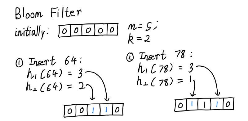
The above diagram illustrates the process of adding the entries to the array. Once the entries have been added, we can do the membership test. Suppose, we test for the membership of element 36. If h1 and h2 produce index 0 and 3, we can easily see that index 0 has not been occupied yet. This means, that for certain the element is not present in the set. However, we may get the index 2 instead of 3, which is already marked as occupied. This may lead us to the wrong conclusion that 36 is present in the set, even though this was never the case. This is a situation of false positives, that is why we say that a bloom filter can only guarantee when an element is not present. If the element is said to be present, there is still the possibility that it might not be, although the probability of such a case can be made quite small by adjusting the values of m and k.
If you’re still not clear, it may help to imagine a bloom filter as a compact checklist with empty boxes. This checklist represents a set that is initially empty. When you add an element to the set, the bloom filter fills in certain boxes based on the element’s characteristics: each element is hashed multiple times using different hash functions which determine which boxes to mark in the checklist. Multiple hash functions ensure that different parts of the checklist are affected, making it more resilient to false positives. When you want to check if an element is in the set, you hash it using the same functions that marked the boxes during insertion. If all the corresponding boxes are marked, the bloom filter suggests that the element might be in the set. However, false positives can occur — the filter might claim an element is in the set when it’s not. False negatives, on the other hand, never happen. If the boxes aren’t marked, the element is definitely not in the set.
As you can see, bloom filters offer speed and efficiency at the expense of some trade-offs. They can produce false positives, but never false negatives. They are fantastic for scenarios where saving memory and quickly filtering out non-members is crucial, but may not be ideal for applications where absolute certainty is required. Now, let’s try to implement them in Python!
Implementing Bloom Filters in Python
Following is the Python implementation of a Bloom Filter.
import hashlib
from bitarray import bitarray

class BloomFilter:
    def __init__(self, size, hash_functions):
        """
        Initialize the Bloom Filter with a given size and number of hash functions.

        :param size: Size of the Bloom Filter (number of bits in the bit array).
        :param hash_functions: Number of hash functions to use.
        """
        self.size = size
        self.bit_array = bitarray(size)
        self.bit_array.setall(0)
        self.hash_functions = hash_functions

    def add(self, item):
        """
        Add an element to the Bloom Filter.

        :param item: The item to be added to the Bloom Filter.
        """
        for i in range(self.hash_functions):
            # Calculate the index using the hash function and update the corresponding bit to 1.
            index = self._hash_function(item, i) % self.size
            self.bit_array[index] = 1

    def contains(self, item):
        """
        Check if an element is likely to be in the Bloom Filter.

        :param item: The item to check for presence in the Bloom Filter.

        :return: True if the element is likely present, False otherwise.
        """
        for i in range(self.hash_functions):
            # Calculate the index using the hash function.
            index = self._hash_function(item, i) % self.size
            # If any corresponding bit is 0, the item is definitely not in the set.
            if not self.bit_array[index]:
                return False
        # If all corresponding bits are 1, the item is likely in the set.
        return True

    def _hash_function(self, item, index):
        """
        To compute the hash function for a given item and index.

        :param item: The item to be hashed.
        :param index: The index used to vary the input to the hash function.

        :return: An integer value obtained by hashing the concatenated string of item and index.
        """
        hash_object = hashlib.sha256()
        hash_object.update((str(item) + str(index)).encode('utf-8'))
        return int.from_bytes(hash_object.digest(), byteorder='big')

# Example usage:
size = 10  # Size of the Bloom Filter
hash_functions = 3  # Number of hash functions

bloom_filter = BloomFilter(size, hash_functions)

# Add elements to the Bloom Filter
bloom_filter.add("apple")
bloom_filter.add("banana")
bloom_filter.add("orange")

# Check if elements are present in the Bloom Filter
print(bloom_filter.contains("apple"))    # True
print(bloom_filter.contains("grape"))    # False (not added)
In the above code, we’ve used the bitarray library for a more memory-efficient representation of the filter. You can install it using: pip3 install bitarray command.
The BloomFilter class is initialized with a specified size (representing the number of bits in the internal bit array) and the number of hash functions to use. The class has methods to add elements to the filter (add) and check for their probable presence (contains). The hash function method is a private function generating hash values based on the SHA-256 algorithm (it’s a good choice since it is known to produce uniformly distributed outputs).
Bloom Filters: Time & Space Complexity Analysis
Let’s also do a quick time and space analysis of bloom filters. In terms of time complexity, both adding elements (add operation) and checking for their probable presence (contains operation) are constant time operations — O(k), where k is the number of hash functions. This is because the filter involves multiple hash functions, each contributing a constant time to the overall process (assuming that hash functions can be evaluated in constant time).
In terms of space complexity, Bloom Filters are memory-efficient since they use a fixed-size bit array. The space required is proportional to the size of the array and the number of hash functions employed. The space complexity is O(m), where m is the size of the bit array. The space efficiency is especially advantageous when dealing with large datasets, as the filter can represent a set of elements using significantly less memory compared to other data structures.
Bloom Filters: The Math
Finally, when it comes to probabilistic data structures, it becomes quintessential to at least propose a bound on the error they can make since they aren’t perfect, unlike their deterministic counterparts. Here, we will go through some math to quantify the probability of making a false positive error and use that to derive meaningful insights.
First, suppose we have an m-sized bit array along with k hash functions. Furthermore, we assume that our hash functions work uniformly, i.e., for any given input they are equally likely to select any of the m lots in the array. Then, the probability of a particular index i being selected is:

Consequently, the probability that the ith index of the bit array is not selected is:

Now, we bring in the k hash functions. We assume that each of them works independently and produces an output. Further, suppose n elements have been already inserted into the array. This means, that the hash functions were used independently for a total of nk times. The probability that the ith index is still empty is therefore:

Thus, the probability that the ith index is occupied is now:

When does a false positive occur? When the index returned by all the elements is 1 even though the element is not present in the set. This happens when the indices produced by all the k hash functions turn out to be occupied. Again, by the independence of the hash function assumption, this amounts to the following probability:

For sufficiently large values of m, we can approximate the above probability into a much simpler expression:

Can we use this to find the optimal value of k that minimizes ε? Sure, it’s just a simple calculus exercise. We simply take the derivative of the above function with respect to k and set it to 0. But, before that, we can simplify the function a bit by taking logarithms on both sides,

This gives us the value of k that minimizes the false positive rate. To ensure that this is really the minimum of the error function, we would ideally want to calculate the second derivative of f(k) and verify our calculation. For the sake of simplicity, we’ve omitted the proof here, but it should be straightforward to show using simple calculus. Next, using the optimal value of k, we can find the minimum value of the error function:

Using the above expression, we can also solve for the optimal value of m:

Okay, that’s a lot of math. Let’s try to understand what and why we’ve done. First, we just used some simple probabilistic expressions to find the probability that the slot at the ith index remains empty after n elements have been inserted using k hash functions. Using this, we obtained the probability of false positive error as a function of n, k, and m. Then, we minimized the function with respect to k. Using this optimal value of k, we found the minimum value of the error function. Solving this for m allows us to determine the minimum size of the bit array such that we can tolerate a given value of error.
Let’s take an example to better gauge these results. Suppose we want to implement a bloom filter and need to find the right values of m and k. We expect about 200,000 elements to be inserted i.e., n = 200000, and the max false positive error we can tolerate is about 1% i.e., ε ̄ = 0.01 Then, the optimal values of m and k can be found as follows:

Using these calculations, we can optimize our original bloom filter implementation:
import math
import hashlib
from bitarray import bitarray

class OptimizedBloomFilter:
    def __init__(self, n=10000, p=0.05):
        """
        Initialize the Optimized Bloom Filter with dynamically calculated parameters.

        :param n: Expected number of elements to be added.
        :param p: Acceptable false positive rate.
        """
        self.n = n
        self.p = p
        self.m, self.k = self._calculate_parameters(n, p)

        self.bit_array = bitarray(self.m)
        self.bit_array.setall(0)

    def add(self, item):
        """
        Add an element to the Optimized Bloom Filter.

        :param item: The item to be added to the Bloom Filter.
        """
        for i in range(self.k):
            index = self._hash_function(item, i) % self.m
            self.bit_array[index] = 1

    def contains(self, item):
        """
        Check if an element is likely to be in the Optimized Bloom Filter.

        :param item: The item to check for presence in the Bloom Filter.

        :return: True if the element is likely present, False otherwise.
        """
        for i in range(self.k):
            index = self._hash_function(item, i) % self.m
            if not self.bit_array[index]:
                return False
        return True

    def _calculate_parameters(self, n, p):
        """
        To calculate the optimal parameters m and k based on n and p.

        :param n: Expected number of elements.
        :param p: Acceptable false positive rate.

        :return: Tuple (m, k) representing the optimal parameters.
        """
        m = - (n * math.log(p)) / (math.log(2) ** 2)
        k = (m / n) * math.log(2)
        return round(m), round(k)

    def _hash_function(self, item, index):
        """
        To compute the hash function for a given item and index.

        :param item: The item to be hashed.
        :param index: The index used to vary the input to the hash function.

        :return: An integer value obtained by hashing the concatenated string of item and index.
        """
        hash_object = hashlib.sha256()
        hash_object.update((str(item) + str(index)).encode('utf-8'))
        return int.from_bytes(hash_object.digest(), byteorder='big')

# Example usage:
expected_elements = 2000000
false_positive_rate = 0.01

optimized_bloom_filter = OptimizedBloomFilter(expected_elements, false_positive_rate)

# Add elements to the Optimized Bloom Filter
optimized_bloom_filter.add("apple")
optimized_bloom_filter.add("banana")
optimized_bloom_filter.add("orange")

# Check if elements are present in the Optimized Bloom Filter
print(optimized_bloom_filter.contains("apple"))    # True
print(optimized_bloom_filter.contains("grape"))    # False (not added)
In this implementation, the OptimizedBloomFilter class dynamically calculates the optimal values for m and k based on the provided expected number of elements (n) and acceptable false positive rate (p). The calculate parameters method handles this calculation. The rest of the implementation remains similar to the previous version, with the optimized parameters improving space efficiency and minimizing the probability of false positives.
This concludes our discussion on bloom filters. Hope you enjoyed reading so far! In the next section, we will discuss another important probabilistic data structure: Count Min Sketch.
Count Min Sketch
In this section, we will discuss another interesting probabilistic data structure: Count Min Sketch. Count Min Sketch is somewhat like an extension of Bloom Filters. Just as the probabilistic counterpart of a hash set is a bloom filter, the counterpart of a multi-set is a count min sketch.
A multi-set is essentially a set that also keeps count of the frequency or number of occurrences of an element in the input data stream. For instance, if input data is [2, 3, 3, 4, 1, 1, 0, 1, 0], a set would simply be the collection of unique elements i.e., {0, 1, 2, 3, 4}. But, a multi-set would also record the frequency, { 0: 2, 1: 3, 2: 1, 3: 3, 4: 1 }, which can be queried as per requirement. A traditional hash table uses the same data structure as a hash set but also records the frequency count of each element. While it is extremely efficient and can be queried in O(1), there may be a large memory cost to store all the elements as well as additional overhead to handle collisions.
Just as before, count min sketch can be much more efficient than the deterministic hash table by significantly reducing the memory requirements and removing the unnecessary computational cost in handling collisions. But, it must pay the price of accuracy, which fortunately can be accounted for by adjusting for the values of m and k as before. Let us take a closer look at how count min sketch works.
How Do They Work?
The core idea behind Count Min Sketch involves using multiple hash functions to map input elements to an array of counters. The array is organized as a two-dimensional matrix, consisting of m columns and k rows with each row corresponding to the hash functions and the columns representing the counters. When an element is encountered in the data stream, it is hashed using each of the hash functions, and the corresponding counters in the matrix are incremented. Due to the nature of hash functions, collisions are inevitable. However, the use of multiple hash functions and a two-dimensional matrix allows Count Min Sketch to distribute the collisions across different counters. This distribution helps in reducing the impact of collisions on the accuracy of the counts.
Suppose, we have an m = 5 (number of columns) and k = 2 (number of rows) hash functions. This means, we only need an array of size m×k = 5×2. Initially, the array is filled with all 0s. Next, we add the elements 2, 3, 2, 2, and 1 to the set. The process is similar to that of a bloom filter. We apply the k hash filters on the input data (the element to be added) and get k indices. Let ji be the output of the ith hash function. Then, we increment the jith index of the ith row by 1. The following figure illustrates how it’s done:

To estimate the frequency of an element, one looks up the counters corresponding to its hashed values and selects the minimum count among them. This minimum count provides an approximation of the true frequency. By repeating this process for multiple elements and taking the minimum counts, one can obtain approximate frequency estimates for various items in the data stream. For instance, if we query for the frequency of 2 in the set, we look at the minimum of 3 and 4 which is 3, and this is indeed the frequency of 2 in the input stream. Similarly, the frequency of 1 is the minimum of 1 and 4, which is 1, again the correct output. It is important to note that count min sketch only provides a maximum bound on the frequency of an element. This bound is derived from the way the algorithm distributes counts across different counters. It may be possible that the indices corresponding to the output of all the k hash functions on the input data might be incremented, not because of the addition of that element per se, but all the other elements in that set. An example is shown below, when we add 4 to the set as well.

Now if we try to query the frequency for 4, we look at the minimum of 4 and 2, which is 2, higher than the actual frequency of 1. This is because the indices corresponding to the output of the hash functions were already filled with those from the other elements due to collisions. The output isn’t perfect, but it is still an upper bound on the actual frequency.
As before, the parameters ’m’ and ’k’ in the Count Min Sketch matrix play a crucial role in balancing memory usage and accuracy. The number of rows ’m’ determines the number of hash functions employed, while the number of columns ’k’ dictates the size of each row and, consequently, the amount of memory used. Adjusting these parameters allows users to control the trade-off between space efficiency and estimation accuracy based on the specific requirements of their application.
Implementing Count Min Sketch in Python
Following is the Python implementation of a Count Min Sketch.
import hashlib

class CountMinSketch:
    def __init__(self, m, k):
        """
        Initialize the Count-Min Sketch with specified width and depth.

        :param width: Number of counters in each hash function's array.
        :param depth: Number of hash functions.
        """
        self.width = m
        self.depth = k
        self.counters = [[0] * m for _ in range(k)]

    def update(self, item, count=1):
        """
        Update the Count-Min Sketch with the occurrence of an item.

        :param item: The item to be counted.
        :param count: The count or frequency of the item (default is 1).
        """
        for i in range(self.depth):
            index = self._hash_function(item, i) % self.width
            self.counters[i][index] += count

    def estimate(self, item):
        """
        Estimate the count or frequency of an item in the Count-Min Sketch.

        :param item: The item to estimate the count for.

        :return: The estimated count of the item.
        """
        min_count = float('inf')
        for i in range(self.depth):
            index = self._hash_function(item, i) % self.width
            min_count = min(min_count, self.counters[i][index])
        return min_count

    def _hash_function(self, item, index):
        """
        To compute the hash function for a given item and index.

        :param item: The item to be hashed.
        :param index: The index used to vary the input to the hash function.

        :return: An integer value obtained by hashing the concatenated string of item and index.
        """
        hash_object = hashlib.sha256()
        hash_object.update((str(item) + str(index)).encode('utf-8'))
        return int.from_bytes(hash_object.digest(), byteorder='big')

# Example usage:
m = 100
k = 5

count_min_sketch = CountMinSketch(m, k)

# Update the sketch with occurrences of items
count_min_sketch.update("apple", 3)
count_min_sketch.update("banana", 5)
count_min_sketch.update("orange", 2)

# Estimate counts for items
print(count_min_sketch.estimate("apple"))    # Estimated count for "apple"
print(count_min_sketch.estimate("grape"))    # Estimated count for "grape" (not updated)
In the above code, the CountMinSketch class is initialized with specified m and k parameters, representing the number of counters in each hash function’s array and the number of hash functions, respectively. The sketch is updated with occurrences of items, and estimates of item counts can be obtained. The hash function method is responsible for generating hash values, and the example usage section demonstrates how to use the Count-Min Sketch to estimate counts for specific items in a streaming fashion. As in the case of bloom filters, the SHA-256 algorithm is used for hashing since it is known to produce uniformly distributed outputs.
Count Min Sketch: Time & Space Complexity Analysis
Let’s also do a quick time and space analysis of the count min sketch. In terms of time complexity, both the addition of elements (incrementing counters) and the estimation of their frequencies in Count Min Sketch are constant time operations: O(k). The constant factor is influenced by the number of hash functions (’k’) and the size of the matrix (’m’). However, assuming that hash functions can be evaluated in constant time, the overall complexity remains constant. The operations involve multiple hash functions, each contributing a constant time to the overall process.
Regarding space complexity, Count Min Sketch is memory-efficient due to its use of a compact matrix structure. The space required is proportional to the product of the number of rows (’m’) and the number of counters per row (’k’). Thus, the space complexity is expressed as O(m * k). We have the flexibility to adjust the values of ’m’ and ’k’ to strike a balance between space efficiency and estimation accuracy. Smaller values result in reduced memory usage but may lead to more estimation errors, while larger values improve accuracy at the expense of increased memory requirements. This tunability makes Count Min Sketch a versatile solution for scenarios where memory constraints are critical, and approximate frequency counts are acceptable.
Count Min Sketch: The Math
As before, using our knowledge of probability theory, we can optimize the count min sketch i.e., find the values of m and k that minimize the possibility of an error. First, let us formalize the notations. Let hat-fₓ denote the frequency estimate for the element x and fₓ denote the actual frequency of that element. Based on our earlier discussion, we must have:

i.e., we are always sure that our estimate is at least the actual frequency count. But is this enough? A stupid algorithm that always outputs a very large number can also achieve this. What makes the count min sketch so special is that we can upper bound not only the actual frequency fₓ but also the deviation of the estimated frequency hat-fₓ from the actual frequency (probabilistic-ally of course). Using an optimal value of m and k, we can guarantee the following:

i.e., the probability that the estimated frequency exceeds the actual frequency by a value of more than or equal to εn (n is the size of the input stream) is at least (1 − δ), where ε and δ can be made as small as required. The values of m and k that satisfy this are as follows:

As we can see, the number of columns (m) controls for the max value of deviation (hat-fₓ −fₓ ), while the number of rows/hash functions (k) controls for the probabilistic guarantee, 1 − δ. The proof of this is quite convoluted and requires some intermediate knowledge of probability theory like random variables and Markov inequality. I will be going through this proof in detail in the following paragraphs. If you’re curious and have the necessary prerequisites, you may continue reading.
So, let’s begin with the proof. First, we define certain quantities: Let αᵢ, ₕᵢ₍ₓ₎ denote the value in the ith row and hᵢ(x) the column of the count min sketch array. This is simply the frequency estimate of x as per the ith row/ith hash function used. This means that the estimated frequency is simply the minimum of this value for all rows:

We now define the random variable Zᵢ (called over-count) as follows:

Next, we define an indicator random variable Xᵢ,ᵧ to check if a collision has occurred in the ith row with some other element y ≠ x. Formally,

Now, let’s think of the relationship between Zᵢ and Xᵢ,ᵧ Recall that Zᵢ is the over-count i.e., the value by which αᵢ, ₕᵢ₍ₓ₎ exceeds the actual frequency fₓ. When does this happen? This happens when there are collisions with elements y ≠ x. This allows us to define the following relation:

Note that we’ve weighted the sum with the actual frequency estimates of y since the elements may occur multiple times, each time causing the overcount to increase. The next step involves finding the expected value of Zᵢ or the over-count using properties of expectation:

where n denotes the expected length of the input stream, which is more than or equal to the sum of the frequencies of all the other elements. Finally, we use Markov’s inequality to find the probability that Zᵢ exceeds its expectation multiplied by a constant:

The above is just the direct use of Markov’s inequality. We may now use the fact that E [Zᵢ] ≤ n/m to get:

Recall the expression we want to prove. All we want on the right-hand side of the inequality in the probability term is εn. Currently, we have an/m. Taking a = mε will allow us to get this term. Therefore,

Now we substitute in m = e/ε to get:

The above must be true for all Zᵢ from i = 1 to i = k. Thus, we can write:

Since the above expression holds for all i, it must also hold for the minimum:

Finally, we take the complement of the above probability and substitute for the value of k:

This completes the proof. From this, we can conclude that to achieve a max deviation of εn with a probabilistic guarantee of 1 − δ, we need the following:

Using these calculations, we can optimize our original count min sketch implementation:
import hashlib
import math

class OptimizedCountMinSketch:
    def __init__(self, epsilon, delta):
        """
        Initialize the Count-Min Sketch with specified width and depth.

        :param epsilon: Quantifies the max deviation from true count (epsilon * n)
        :param delta: To compute the probabilistic guarantee
        """
        self.epsilon = epsilon
        self.delta = delta
        self.width, self.depth = self._calculate_parameters(epsilon, delta)
        self.counters = [[0] * self.width for _ in range(self.depth)]

    def update(self, item, count=1):
        """
        Update the Count-Min Sketch with the occurrence of an item.

        :param item: The item to be counted.
        :param count: The count or frequency of the item (default is 1).
        """
        for i in range(self.depth):
            index = self._hash_function(item, i) % self.width
            self.counters[i][index] += count

    def estimate(self, item):
        """
        Estimate the count or frequency of an item in the Count-Min Sketch.

        :param item: The item to estimate the count for.

        :return: The estimated count of the item.
        """
        min_count = float('inf')
        for i in range(self.depth):
            index = self._hash_function(item, i) % self.width
            min_count = min(min_count, self.counters[i][index])
        return min_count

    def _calculate_parameters(self, epsilon, delta):
        """
        To calculate the optimal parameters m and k based on s and e.

        :param epsilon: Quantifies the max deviation from true count (epsilon * n)
        :param delta: To compute the probabilistic guarantee

        :return: Tuple (m, k) representing the optimal parameters.
        """
        m = math.ceil(math.e/epsilon)
        k = math.ceil(math.log(1/delta))
        return m, k

    def _hash_function(self, item, index):
        """
        To compute the hash function for a given item and index.

        :param item: The item to be hashed.
        :param index: The index used to vary the input to the hash function.

        :return: An integer value obtained by hashing the concatenated string of item and index.
        """
        hash_object = hashlib.sha256()
        hash_object.update((str(item) + str(index)).encode('utf-8'))
        return int.from_bytes(hash_object.digest(), byteorder='big')

# Example usage:
eps = 0.01
delta = 0.05

optimized_count_min_sketch = OptimizedCountMinSketch(eps, delta)

# Update the sketch with occurrences of items
optimized_count_min_sketch.update("apple", 3)
optimized_count_min_sketch.update("banana", 5)
optimized_count_min_sketch.update("orange", 2)

# Estimate counts for items
print(count_min_sketch.estimate("apple"))    # Estimated count for "apple"
print(count_min_sketch.estimate("grape"))    # Estimated count for "grape" (not updated)
In this implementation, the OptimizedCountMinSketch class dynamically calculates the optimal values for m and k based on the provided max deviation tolerance (epsilon) and probabilistic requirement (delta). The calculate parameters method handles this calculation. The rest of the implementation remains similar to the previous version, with the optimized parameters achieving the required guarantee.
This concludes our discussion on Count Min Sketch.
The Bottom Line
Donald Knuth, the father of the analysis of algorithms had said,
“An algorithm must be seen to be believed”.
Indeed, the ability to appreciate an algorithm comes, not only from using it, but understanding how it works and why it works. In this article, I’ve tried to describe the inner workings of two important probabilistic data structures and their algorithms. We talked about their performance relative to their deterministic counterparts, and implementation, as well as used some math to quantify their error bound. Although quite important in literature, these data structures merely constitute the surface of an ocean of other probabilistic data structures such as skip lists, hyper log-log, treap, quotient filter, min hash, etc. Many of these are very interesting and have a lot of potential applications in the field of computer science. I hope to go through some of these in further detail in my subsequent articles.
Hope you enjoyed reading this article! In case you have any doubts or suggestions, do reply in the comment box. Please feel free to contact me via mail.
If you liked my article and want to read more of them, please follow me.
Note: All images (except for the cover image) have been made by the author.
References
- Bloom filter — Wikipedia — en.wikipedia.org. https://en.wikipedia.org/wiki/Bloom_filter. [Accessed 07–01- 2024].
- Bloom Filters — Introduction and Implementation — GeeksforGeeks — geeksforgeeks.org. https://www. geeksforgeeks.org/bloom-filters-introduction-and-python-implementation/. [Accessed 07–01–2024].
- Count-Min Sketch Data Structure with Implementation — GeeksforGeeks — geeksforgeeks.org. https://www. geeksforgeeks.org/count-min-sketch-in-java-with-examples/. [Accessed 07–01–2024].
- Counting Bloom Filters — Introduction and Implementation — GeeksforGeeks — geeksforgeeks.org. https://www. geeksforgeeks.org/counting-bloom-filters-introduction-and-implementation/. [Accessed 07–01–2024].
- Count–min sketch — Wikipedia — en.wikipedia.org. https://en.wikipedia.org/wiki/Count%E2%80%93min_sketch. [Accessed 07–01–2024].
- Humberto Villalta. Bloom Filter Mathematical Proof — humberto521336. https://medium.com/@humberto521336/ bloom-filters-mathematical-proof-8aa2e5d7b06b. [Accessed 07–01–2024].
Probabilistic Data Structures Decoded: Enhancing Performance in Modern Computing was originally published in Towards Data Science on Medium, where people are continuing the conversation by highlighting and responding to this story.
The Ultimate Guide to Understanding and Implementing Bloom Filters and Count Min Sketch in Python

Contents
- Introduction
- What is a Probabilistic Data Structure?
- Bloom Filters
3.1 How Do They Work
3.2 Implementing Bloom Filters in Python
3.3 Bloom Filters: Time & Space Complexity Analysis
3.4 Bloom Filters: The Math - Count Min Sketch
3.1 How Do They Work
3.2 Implementing Count Min Sketch in Python
3.3 Count Min Sketch: Time & Space Complexity Analysis
3.4 Count Min Sketch: The Math - The Bottom Line
- References
Note: The entire code file used in this article is available at the following repository: https://github.com/namanlab/Probabilistic_Data_Structures
Introduction
Computer science enthusiasts often find themselves enamored by the subtle charm of algorithms — the silent workhorses that streamline our digital interactions. At its core, programming is all about getting tasks done through the use of efficient algorithms synchronized with optimal data structures. That’s why there’s a whole field in Computer Science dedicated to the design and analysis of algorithms given their role as the architects of the digital age, quietly shaping our technological experiences with a blend of logic and precision.
A traditional curriculum in data structures and algorithms often exposes students to some of the fundamental data structures (deterministic) such as Arrays, Linked Lists, Stacks and Queues, Binary Search Trees, AVL trees, Heaps, Hash Maps, and of course Graphs. Indeed, the study of such data structures and the associated algorithms constitutes the foundation for the development of much more sophisticated programs aimed at solving a variety of tasks. In this article, I will introduce probabilistic data structures such as Bloom Filters and Count-Min Sketch, some of the lesser-known data structures. While some introductory courses do talk about a few of these briefly, they constitute a subset of those data structures that are often neglected, yet come out as important ideas in various academic discussions. In this article, we will describe what probabilistic data structures are, their significance, examples, and their implementation, as well as go through some of the math required to better gauge their performance. Let’s begin!
What is a Probabilistic Data Structure?
Probabilistic data structures are clever tools in computer science that provide fast and memory-efficient approximations of certain operations. Unlike deterministic data structures, which always give precise and accurate results, probabilistic ones sacrifice a bit of accuracy for added efficiency. In simple terms, these structures use randomness to quickly estimate answers to questions without storing all the exact details; somewhat like smart shortcuts, making educated guesses rather than doing the full work.
Take the example of a bloom filter, a probabilistic data structure quite similar to HashSet. It helps you check whether an element is likely in a set or definitely not. It might say ”possibly in the set” or ”definitely not in the set,” but it won’t guarantee ”definitely in the set.” This uncertainty allows it to be fast and save a lot more memory than a traditional hash set.
Deterministic data structures such as linked lists and AVL trees that we commonly encounter, on the other hand, give you 100% sure answers. For example, if you ask whether an element is in a hash set, it’ll say ”yes” or ”no” without any doubt. However, this certainty often comes at the cost of using more memory or taking longer to process.
The over-arching idea is that probabilistic data structures trade a bit of accuracy for speed and efficiency, making them handy in situations where you can tolerate a small chance of error. They’re like quick and savvy assistants that provide close-to-perfect answers without doing all the heavy lifting. Imagine you have a huge collection of data and want to perform operations like searching, inserting, or checking membership. Deterministic structures guarantee correctness but may become sluggish when dealing with massive datasets. Probabilistic structures, by embracing a bit of uncertainty, provide a way to handle these tasks swiftly and with reduced memory requirements. For the rest of this article, we will explore some of the commonly used probabilistic data structures: Bloom Filters and Count-Min Sketch. Let’s start with Bloom Filters!
Bloom Filters
Bloom filters are designed for quick and memory-efficient membership tests i.e., they help answer the question: ”Is this element a member of a set?” They are particularly handy in scenarios where speed and resource conservation are critical, such as database lookups, network routers, and caching systems.
How Do They Work?
A bloom filter is implemented as an m-sized bit array, which is just an array of size m that is filled with either 0 or 1. An empty bloom filter is initially filled with all 0s. Whenever an element is added, a set of hash functions maps the element to a set of indices. A hash function is a function that transforms input data of any size into a small integer (called a hash code or hash value) that can be used as the index.
Recall, how a traditional hash set works. A traditional hash set applies just one hash function on the input data (the element to be added to the set) and produces a hash code corresponding to the index to which the element is added to the table. While this approach provides a simple and fast way to organize and retrieve data (usually in constant, O(1) time), it comes with inherent memory inefficiencies, primarily related to collisions and fixed-size tables.
The use of a single hash function can lead to collisions, where different elements produce the same hash code and attempt to occupy the same index in the hash table. This affects the efficiency of the hash set, as it necessitates additional mechanisms to handle and resolve such conflicts. Moreover, the fixed size of the hash table leads to inefficiencies in adapting to varying workloads. As the number of elements increases or decreases, the load factor (the ratio of elements to the table size) may become unfavorable. This can lead to increased collisions and degradation of performance. To counter this, hash sets often need to be resized, a process that involves creating a new, larger table and rehashing all existing elements. This operation, while necessary, introduces additional computational overhead and memory requirements.
A bloom filter on the other hand doesn’t need such a large table, it can do the job with a smaller m-sized array and through the use of multiple hash functions (say, k different hash functions) instead of just a single one. The filter works by applying all the k hash functions on the input data and marking all the k output indices as 1 in the original array. Here’s an example to show how it works.
Suppose, we have an m = 5-bit sized array initially filled with 0s and k = 2 hash functions. Usually, the hash functions we use must satisfy two key properties: i) they should be fast to compute, and ii) the output should be more or less uniformly distributed to minimize the risk of false positives (don’t worry, details will be discussed later). Next, we add the elements 64 and 78 to the array.
The above diagram illustrates the process of adding the entries to the array. Once the entries have been added, we can do the membership test. Suppose, we test for the membership of element 36. If h1 and h2 produce index 0 and 3, we can easily see that index 0 has not been occupied yet. This means, that for certain the element is not present in the set. However, we may get the index 2 instead of 3, which is already marked as occupied. This may lead us to the wrong conclusion that 36 is present in the set, even though this was never the case. This is a situation of false positives, that is why we say that a bloom filter can only guarantee when an element is not present. If the element is said to be present, there is still the possibility that it might not be, although the probability of such a case can be made quite small by adjusting the values of m and k.
If you’re still not clear, it may help to imagine a bloom filter as a compact checklist with empty boxes. This checklist represents a set that is initially empty. When you add an element to the set, the bloom filter fills in certain boxes based on the element’s characteristics: each element is hashed multiple times using different hash functions which determine which boxes to mark in the checklist. Multiple hash functions ensure that different parts of the checklist are affected, making it more resilient to false positives. When you want to check if an element is in the set, you hash it using the same functions that marked the boxes during insertion. If all the corresponding boxes are marked, the bloom filter suggests that the element might be in the set. However, false positives can occur — the filter might claim an element is in the set when it’s not. False negatives, on the other hand, never happen. If the boxes aren’t marked, the element is definitely not in the set.
As you can see, bloom filters offer speed and efficiency at the expense of some trade-offs. They can produce false positives, but never false negatives. They are fantastic for scenarios where saving memory and quickly filtering out non-members is crucial, but may not be ideal for applications where absolute certainty is required. Now, let’s try to implement them in Python!
Implementing Bloom Filters in Python
Following is the Python implementation of a Bloom Filter.
import hashlib
from bitarray import bitarray

class BloomFilter:
    def __init__(self, size, hash_functions):
        """
        Initialize the Bloom Filter with a given size and number of hash functions.

        :param size: Size of the Bloom Filter (number of bits in the bit array).
        :param hash_functions: Number of hash functions to use.
        """
        self.size = size
        self.bit_array = bitarray(size)
        self.bit_array.setall(0)
        self.hash_functions = hash_functions

    def add(self, item):
        """
        Add an element to the Bloom Filter.

        :param item: The item to be added to the Bloom Filter.
        """
        for i in range(self.hash_functions):
            # Calculate the index using the hash function and update the corresponding bit to 1.
            index = self._hash_function(item, i) % self.size
            self.bit_array[index] = 1

    def contains(self, item):
        """
        Check if an element is likely to be in the Bloom Filter.

        :param item: The item to check for presence in the Bloom Filter.

        :return: True if the element is likely present, False otherwise.
        """
        for i in range(self.hash_functions):
            # Calculate the index using the hash function.
            index = self._hash_function(item, i) % self.size
            # If any corresponding bit is 0, the item is definitely not in the set.
            if not self.bit_array[index]:
                return False
        # If all corresponding bits are 1, the item is likely in the set.
        return True

    def _hash_function(self, item, index):
        """
        To compute the hash function for a given item and index.

        :param item: The item to be hashed.
        :param index: The index used to vary the input to the hash function.

        :return: An integer value obtained by hashing the concatenated string of item and index.
        """
        hash_object = hashlib.sha256()
        hash_object.update((str(item) + str(index)).encode('utf-8'))
        return int.from_bytes(hash_object.digest(), byteorder='big')

# Example usage:
size = 10  # Size of the Bloom Filter
hash_functions = 3  # Number of hash functions

bloom_filter = BloomFilter(size, hash_functions)

# Add elements to the Bloom Filter
bloom_filter.add("apple")
bloom_filter.add("banana")
bloom_filter.add("orange")

# Check if elements are present in the Bloom Filter
print(bloom_filter.contains("apple"))    # True
print(bloom_filter.contains("grape"))    # False (not added)
In the above code, we’ve used the bitarray library for a more memory-efficient representation of the filter. You can install it using: pip3 install bitarray command.
The BloomFilter class is initialized with a specified size (representing the number of bits in the internal bit array) and the number of hash functions to use. The class has methods to add elements to the filter (add) and check for their probable presence (contains). The hash function method is a private function generating hash values based on the SHA-256 algorithm (it’s a good choice since it is known to produce uniformly distributed outputs).
Bloom Filters: Time & Space Complexity Analysis
Let’s also do a quick time and space analysis of bloom filters. In terms of time complexity, both adding elements (add operation) and checking for their probable presence (contains operation) are constant time operations — O(k), where k is the number of hash functions. This is because the filter involves multiple hash functions, each contributing a constant time to the overall process (assuming that hash functions can be evaluated in constant time).
In terms of space complexity, Bloom Filters are memory-efficient since they use a fixed-size bit array. The space required is proportional to the size of the array and the number of hash functions employed. The space complexity is O(m), where m is the size of the bit array. The space efficiency is especially advantageous when dealing with large datasets, as the filter can represent a set of elements using significantly less memory compared to other data structures.
Bloom Filters: The Math
Finally, when it comes to probabilistic data structures, it becomes quintessential to at least propose a bound on the error they can make since they aren’t perfect, unlike their deterministic counterparts. Here, we will go through some math to quantify the probability of making a false positive error and use that to derive meaningful insights.
First, suppose we have an m-sized bit array along with k hash functions. Furthermore, we assume that our hash functions work uniformly, i.e., for any given input they are equally likely to select any of the m lots in the array. Then, the probability of a particular index i being selected is:
Consequently, the probability that the ith index of the bit array is not selected is:
Now, we bring in the k hash functions. We assume that each of them works independently and produces an output. Further, suppose n elements have been already inserted into the array. This means, that the hash functions were used independently for a total of nk times. The probability that the ith index is still empty is therefore:
Thus, the probability that the ith index is occupied is now:
When does a false positive occur? When the index returned by all the elements is 1 even though the element is not present in the set. This happens when the indices produced by all the k hash functions turn out to be occupied. Again, by the independence of the hash function assumption, this amounts to the following probability:
For sufficiently large values of m, we can approximate the above probability into a much simpler expression:
Can we use this to find the optimal value of k that minimizes ε? Sure, it’s just a simple calculus exercise. We simply take the derivative of the above function with respect to k and set it to 0. But, before that, we can simplify the function a bit by taking logarithms on both sides,
This gives us the value of k that minimizes the false positive rate. To ensure that this is really the minimum of the error function, we would ideally want to calculate the second derivative of f(k) and verify our calculation. For the sake of simplicity, we’ve omitted the proof here, but it should be straightforward to show using simple calculus. Next, using the optimal value of k, we can find the minimum value of the error function:
Using the above expression, we can also solve for the optimal value of m:
Okay, that’s a lot of math. Let’s try to understand what and why we’ve done. First, we just used some simple probabilistic expressions to find the probability that the slot at the ith index remains empty after n elements have been inserted using k hash functions. Using this, we obtained the probability of false positive error as a function of n, k, and m. Then, we minimized the function with respect to k. Using this optimal value of k, we found the minimum value of the error function. Solving this for m allows us to determine the minimum size of the bit array such that we can tolerate a given value of error.
Let’s take an example to better gauge these results. Suppose we want to implement a bloom filter and need to find the right values of m and k. We expect about 200,000 elements to be inserted i.e., n = 200000, and the max false positive error we can tolerate is about 1% i.e., ε ̄ = 0.01 Then, the optimal values of m and k can be found as follows:
Using these calculations, we can optimize our original bloom filter implementation:
import math
import hashlib
from bitarray import bitarray

class OptimizedBloomFilter:
    def __init__(self, n=10000, p=0.05):
        """
        Initialize the Optimized Bloom Filter with dynamically calculated parameters.

        :param n: Expected number of elements to be added.
        :param p: Acceptable false positive rate.
        """
        self.n = n
        self.p = p
        self.m, self.k = self._calculate_parameters(n, p)

        self.bit_array = bitarray(self.m)
        self.bit_array.setall(0)

    def add(self, item):
        """
        Add an element to the Optimized Bloom Filter.

        :param item: The item to be added to the Bloom Filter.
        """
        for i in range(self.k):
            index = self._hash_function(item, i) % self.m
            self.bit_array[index] = 1

    def contains(self, item):
        """
        Check if an element is likely to be in the Optimized Bloom Filter.

        :param item: The item to check for presence in the Bloom Filter.

        :return: True if the element is likely present, False otherwise.
        """
        for i in range(self.k):
            index = self._hash_function(item, i) % self.m
            if not self.bit_array[index]:
                return False
        return True

    def _calculate_parameters(self, n, p):
        """
        To calculate the optimal parameters m and k based on n and p.

        :param n: Expected number of elements.
        :param p: Acceptable false positive rate.

        :return: Tuple (m, k) representing the optimal parameters.
        """
        m = - (n * math.log(p)) / (math.log(2) ** 2)
        k = (m / n) * math.log(2)
        return round(m), round(k)

    def _hash_function(self, item, index):
        """
        To compute the hash function for a given item and index.

        :param item: The item to be hashed.
        :param index: The index used to vary the input to the hash function.

        :return: An integer value obtained by hashing the concatenated string of item and index.
        """
        hash_object = hashlib.sha256()
        hash_object.update((str(item) + str(index)).encode('utf-8'))
        return int.from_bytes(hash_object.digest(), byteorder='big')

# Example usage:
expected_elements = 2000000
false_positive_rate = 0.01

optimized_bloom_filter = OptimizedBloomFilter(expected_elements, false_positive_rate)

# Add elements to the Optimized Bloom Filter
optimized_bloom_filter.add("apple")
optimized_bloom_filter.add("banana")
optimized_bloom_filter.add("orange")

# Check if elements are present in the Optimized Bloom Filter
print(optimized_bloom_filter.contains("apple"))    # True
print(optimized_bloom_filter.contains("grape"))    # False (not added)
In this implementation, the OptimizedBloomFilter class dynamically calculates the optimal values for m and k based on the provided expected number of elements (n) and acceptable false positive rate (p). The calculate parameters method handles this calculation. The rest of the implementation remains similar to the previous version, with the optimized parameters improving space efficiency and minimizing the probability of false positives.
This concludes our discussion on bloom filters. Hope you enjoyed reading so far! In the next section, we will discuss another important probabilistic data structure: Count Min Sketch.
Count Min Sketch
In this section, we will discuss another interesting probabilistic data structure: Count Min Sketch. Count Min Sketch is somewhat like an extension of Bloom Filters. Just as the probabilistic counterpart of a hash set is a bloom filter, the counterpart of a multi-set is a count min sketch.
A multi-set is essentially a set that also keeps count of the frequency or number of occurrences of an element in the input data stream. For instance, if input data is [2, 3, 3, 4, 1, 1, 0, 1, 0], a set would simply be the collection of unique elements i.e., {0, 1, 2, 3, 4}. But, a multi-set would also record the frequency, { 0: 2, 1: 3, 2: 1, 3: 3, 4: 1 }, which can be queried as per requirement. A traditional hash table uses the same data structure as a hash set but also records the frequency count of each element. While it is extremely efficient and can be queried in O(1), there may be a large memory cost to store all the elements as well as additional overhead to handle collisions.
Just as before, count min sketch can be much more efficient than the deterministic hash table by significantly reducing the memory requirements and removing the unnecessary computational cost in handling collisions. But, it must pay the price of accuracy, which fortunately can be accounted for by adjusting for the values of m and k as before. Let us take a closer look at how count min sketch works.
How Do They Work?
The core idea behind Count Min Sketch involves using multiple hash functions to map input elements to an array of counters. The array is organized as a two-dimensional matrix, consisting of m columns and k rows with each row corresponding to the hash functions and the columns representing the counters. When an element is encountered in the data stream, it is hashed using each of the hash functions, and the corresponding counters in the matrix are incremented. Due to the nature of hash functions, collisions are inevitable. However, the use of multiple hash functions and a two-dimensional matrix allows Count Min Sketch to distribute the collisions across different counters. This distribution helps in reducing the impact of collisions on the accuracy of the counts.
Suppose, we have an m = 5 (number of columns) and k = 2 (number of rows) hash functions. This means, we only need an array of size m×k = 5×2. Initially, the array is filled with all 0s. Next, we add the elements 2, 3, 2, 2, and 1 to the set. The process is similar to that of a bloom filter. We apply the k hash filters on the input data (the element to be added) and get k indices. Let ji be the output of the ith hash function. Then, we increment the jith index of the ith row by 1. The following figure illustrates how it’s done:
To estimate the frequency of an element, one looks up the counters corresponding to its hashed values and selects the minimum count among them. This minimum count provides an approximation of the true frequency. By repeating this process for multiple elements and taking the minimum counts, one can obtain approximate frequency estimates for various items in the data stream. For instance, if we query for the frequency of 2 in the set, we look at the minimum of 3 and 4 which is 3, and this is indeed the frequency of 2 in the input stream. Similarly, the frequency of 1 is the minimum of 1 and 4, which is 1, again the correct output. It is important to note that count min sketch only provides a maximum bound on the frequency of an element. This bound is derived from the way the algorithm distributes counts across different counters. It may be possible that the indices corresponding to the output of all the k hash functions on the input data might be incremented, not because of the addition of that element per se, but all the other elements in that set. An example is shown below, when we add 4 to the set as well.
Now if we try to query the frequency for 4, we look at the minimum of 4 and 2, which is 2, higher than the actual frequency of 1. This is because the indices corresponding to the output of the hash functions were already filled with those from the other elements due to collisions. The output isn’t perfect, but it is still an upper bound on the actual frequency.
As before, the parameters ’m’ and ’k’ in the Count Min Sketch matrix play a crucial role in balancing memory usage and accuracy. The number of rows ’m’ determines the number of hash functions employed, while the number of columns ’k’ dictates the size of each row and, consequently, the amount of memory used. Adjusting these parameters allows users to control the trade-off between space efficiency and estimation accuracy based on the specific requirements of their application.
Implementing Count Min Sketch in Python
Following is the Python implementation of a Count Min Sketch.
import hashlib

class CountMinSketch:
    def __init__(self, m, k):
        """
        Initialize the Count-Min Sketch with specified width and depth.

        :param width: Number of counters in each hash function's array.
        :param depth: Number of hash functions.
        """
        self.width = m
        self.depth = k
        self.counters = [[0] * m for _ in range(k)]

    def update(self, item, count=1):
        """
        Update the Count-Min Sketch with the occurrence of an item.

        :param item: The item to be counted.
        :param count: The count or frequency of the item (default is 1).
        """
        for i in range(self.depth):
            index = self._hash_function(item, i) % self.width
            self.counters[i][index] += count

    def estimate(self, item):
        """
        Estimate the count or frequency of an item in the Count-Min Sketch.

        :param item: The item to estimate the count for.

        :return: The estimated count of the item.
        """
        min_count = float('inf')
        for i in range(self.depth):
            index = self._hash_function(item, i) % self.width
            min_count = min(min_count, self.counters[i][index])
        return min_count

    def _hash_function(self, item, index):
        """
        To compute the hash function for a given item and index.

        :param item: The item to be hashed.
        :param index: The index used to vary the input to the hash function.

        :return: An integer value obtained by hashing the concatenated string of item and index.
        """
        hash_object = hashlib.sha256()
        hash_object.update((str(item) + str(index)).encode('utf-8'))
        return int.from_bytes(hash_object.digest(), byteorder='big')

# Example usage:
m = 100
k = 5

count_min_sketch = CountMinSketch(m, k)

# Update the sketch with occurrences of items
count_min_sketch.update("apple", 3)
count_min_sketch.update("banana", 5)
count_min_sketch.update("orange", 2)

# Estimate counts for items
print(count_min_sketch.estimate("apple"))    # Estimated count for "apple"
print(count_min_sketch.estimate("grape"))    # Estimated count for "grape" (not updated)
In the above code, the CountMinSketch class is initialized with specified m and k parameters, representing the number of counters in each hash function’s array and the number of hash functions, respectively. The sketch is updated with occurrences of items, and estimates of item counts can be obtained. The hash function method is responsible for generating hash values, and the example usage section demonstrates how to use the Count-Min Sketch to estimate counts for specific items in a streaming fashion. As in the case of bloom filters, the SHA-256 algorithm is used for hashing since it is known to produce uniformly distributed outputs.
Count Min Sketch: Time & Space Complexity Analysis
Let’s also do a quick time and space analysis of the count min sketch. In terms of time complexity, both the addition of elements (incrementing counters) and the estimation of their frequencies in Count Min Sketch are constant time operations: O(k). The constant factor is influenced by the number of hash functions (’k’) and the size of the matrix (’m’). However, assuming that hash functions can be evaluated in constant time, the overall complexity remains constant. The operations involve multiple hash functions, each contributing a constant time to the overall process.
Regarding space complexity, Count Min Sketch is memory-efficient due to its use of a compact matrix structure. The space required is proportional to the product of the number of rows (’m’) and the number of counters per row (’k’). Thus, the space complexity is expressed as O(m * k). We have the flexibility to adjust the values of ’m’ and ’k’ to strike a balance between space efficiency and estimation accuracy. Smaller values result in reduced memory usage but may lead to more estimation errors, while larger values improve accuracy at the expense of increased memory requirements. This tunability makes Count Min Sketch a versatile solution for scenarios where memory constraints are critical, and approximate frequency counts are acceptable.
Count Min Sketch: The Math
As before, using our knowledge of probability theory, we can optimize the count min sketch i.e., find the values of m and k that minimize the possibility of an error. First, let us formalize the notations. Let hat-fₓ denote the frequency estimate for the element x and fₓ denote the actual frequency of that element. Based on our earlier discussion, we must have:
i.e., we are always sure that our estimate is at least the actual frequency count. But is this enough? A stupid algorithm that always outputs a very large number can also achieve this. What makes the count min sketch so special is that we can upper bound not only the actual frequency fₓ but also the deviation of the estimated frequency hat-fₓ from the actual frequency (probabilistic-ally of course). Using an optimal value of m and k, we can guarantee the following:
i.e., the probability that the estimated frequency exceeds the actual frequency by a value of more than or equal to εn (n is the size of the input stream) is at least (1 − δ), where ε and δ can be made as small as required. The values of m and k that satisfy this are as follows:
As we can see, the number of columns (m) controls for the max value of deviation (hat-fₓ −fₓ ), while the number of rows/hash functions (k) controls for the probabilistic guarantee, 1 − δ. The proof of this is quite convoluted and requires some intermediate knowledge of probability theory like random variables and Markov inequality. I will be going through this proof in detail in the following paragraphs. If you’re curious and have the necessary prerequisites, you may continue reading.
So, let’s begin with the proof. First, we define certain quantities: Let αᵢ, ₕᵢ₍ₓ₎ denote the value in the ith row and hᵢ(x) the column of the count min sketch array. This is simply the frequency estimate of x as per the ith row/ith hash function used. This means that the estimated frequency is simply the minimum of this value for all rows:
We now define the random variable Zᵢ (called over-count) as follows:
Next, we define an indicator random variable Xᵢ,ᵧ to check if a collision has occurred in the ith row with some other element y ≠ x. Formally,
Now, let’s think of the relationship between Zᵢ and Xᵢ,ᵧ Recall that Zᵢ is the over-count i.e., the value by which αᵢ, ₕᵢ₍ₓ₎ exceeds the actual frequency fₓ. When does this happen? This happens when there are collisions with elements y ≠ x. This allows us to define the following relation:
Note that we’ve weighted the sum with the actual frequency estimates of y since the elements may occur multiple times, each time causing the overcount to increase. The next step involves finding the expected value of Zᵢ or the over-count using properties of expectation:
where n denotes the expected length of the input stream, which is more than or equal to the sum of the frequencies of all the other elements. Finally, we use Markov’s inequality to find the probability that Zᵢ exceeds its expectation multiplied by a constant:
The above is just the direct use of Markov’s inequality. We may now use the fact that E [Zᵢ] ≤ n/m to get:
Recall the expression we want to prove. All we want on the right-hand side of the inequality in the probability term is εn. Currently, we have an/m. Taking a = mε will allow us to get this term. Therefore,
Now we substitute in m = e/ε to get:
The above must be true for all Zᵢ from i = 1 to i = k. Thus, we can write:
Since the above expression holds for all i, it must also hold for the minimum:
Finally, we take the complement of the above probability and substitute for the value of k:
This completes the proof. From this, we can conclude that to achieve a max deviation of εn with a probabilistic guarantee of 1 − δ, we need the following:
Using these calculations, we can optimize our original count min sketch implementation:
import hashlib
import math

class OptimizedCountMinSketch:
    def __init__(self, epsilon, delta):
        """
        Initialize the Count-Min Sketch with specified width and depth.

        :param epsilon: Quantifies the max deviation from true count (epsilon * n)
        :param delta: To compute the probabilistic guarantee
        """
        self.epsilon = epsilon
        self.delta = delta
        self.width, self.depth = self._calculate_parameters(epsilon, delta)
        self.counters = [[0] * self.width for _ in range(self.depth)]

    def update(self, item, count=1):
        """
        Update the Count-Min Sketch with the occurrence of an item.

        :param item: The item to be counted.
        :param count: The count or frequency of the item (default is 1).
        """
        for i in range(self.depth):
            index = self._hash_function(item, i) % self.width
            self.counters[i][index] += count

    def estimate(self, item):
        """
        Estimate the count or frequency of an item in the Count-Min Sketch.

        :param item: The item to estimate the count for.

        :return: The estimated count of the item.
        """
        min_count = float('inf')
        for i in range(self.depth):
            index = self._hash_function(item, i) % self.width
            min_count = min(min_count, self.counters[i][index])
        return min_count

    def _calculate_parameters(self, epsilon, delta):
        """
        To calculate the optimal parameters m and k based on s and e.

        :param epsilon: Quantifies the max deviation from true count (epsilon * n)
        :param delta: To compute the probabilistic guarantee

        :return: Tuple (m, k) representing the optimal parameters.
        """
        m = math.ceil(math.e/epsilon)
        k = math.ceil(math.log(1/delta))
        return m, k

    def _hash_function(self, item, index):
        """
        To compute the hash function for a given item and index.

        :param item: The item to be hashed.
        :param index: The index used to vary the input to the hash function.

        :return: An integer value obtained by hashing the concatenated string of item and index.
        """
        hash_object = hashlib.sha256()
        hash_object.update((str(item) + str(index)).encode('utf-8'))
        return int.from_bytes(hash_object.digest(), byteorder='big')

# Example usage:
eps = 0.01
delta = 0.05

optimized_count_min_sketch = OptimizedCountMinSketch(eps, delta)

# Update the sketch with occurrences of items
optimized_count_min_sketch.update("apple", 3)
optimized_count_min_sketch.update("banana", 5)
optimized_count_min_sketch.update("orange", 2)

# Estimate counts for items
print(count_min_sketch.estimate("apple"))    # Estimated count for "apple"
print(count_min_sketch.estimate("grape"))    # Estimated count for "grape" (not updated)
In this implementation, the OptimizedCountMinSketch class dynamically calculates the optimal values for m and k based on the provided max deviation tolerance (epsilon) and probabilistic requirement (delta). The calculate parameters method handles this calculation. The rest of the implementation remains similar to the previous version, with the optimized parameters achieving the required guarantee.
This concludes our discussion on Count Min Sketch.
The Bottom Line
Donald Knuth, the father of the analysis of algorithms had said,
“An algorithm must be seen to be believed”.
Indeed, the ability to appreciate an algorithm comes, not only from using it, but understanding how it works and why it works. In this article, I’ve tried to describe the inner workings of two important probabilistic data structures and their algorithms. We talked about their performance relative to their deterministic counterparts, and implementation, as well as used some math to quantify their error bound. Although quite important in literature, these data structures merely constitute the surface of an ocean of other probabilistic data structures such as skip lists, hyper log-log, treap, quotient filter, min hash, etc. Many of these are very interesting and have a lot of potential applications in the field of computer science. I hope to go through some of these in further detail in my subsequent articles.
Hope you enjoyed reading this article! In case you have any doubts or suggestions, do reply in the comment box. Please feel free to contact me via mail.
If you liked my article and want to read more of them, please follow me.
Note: All images (except for the cover image) have been made by the author.
References
- Bloom filter — Wikipedia — en.wikipedia.org. https://en.wikipedia.org/wiki/Bloom_filter. [Accessed 07–01- 2024].
- Bloom Filters — Introduction and Implementation — GeeksforGeeks — geeksforgeeks.org. https://www. geeksforgeeks.org/bloom-filters-introduction-and-python-implementation/. [Accessed 07–01–2024].
- Count-Min Sketch Data Structure with Implementation — GeeksforGeeks — geeksforgeeks.org. https://www. geeksforgeeks.org/count-min-sketch-in-java-with-examples/. [Accessed 07–01–2024].
- Counting Bloom Filters — Introduction and Implementation — GeeksforGeeks — geeksforgeeks.org. https://www. geeksforgeeks.org/counting-bloom-filters-introduction-and-implementation/. [Accessed 07–01–2024].
- Count–min sketch — Wikipedia — en.wikipedia.org. https://en.wikipedia.org/wiki/Count%E2%80%93min_sketch. [Accessed 07–01–2024].
- Humberto Villalta. Bloom Filter Mathematical Proof — humberto521336. https://medium.com/@humberto521336/ bloom-filters-mathematical-proof-8aa2e5d7b06b. [Accessed 07–01–2024].
Probabilistic Data Structures Decoded: Enhancing Performance in Modern Computing was originally published in Towards Data Science on Medium, where people are continuing the conversation by highlighting and responding to this story.
Denial of responsibility! Techno Blender is an automatic aggregator of the all world’s media. In each content, the hyperlink to the primary source is specified. All trademarks belong to their rightful owners, all materials to their authors. If you are the owner of the content and do not want us to publish your materials, please contact us by email – [email protected]. The content will be deleted within 24 hours.