
RAG: How to Talk to Your Data
Comprehensive guide on how to analyse customer feedback using ChatGPT
In my previous articles, we discussed how to do Topic Modelling using ChatGPT. Our task was to analyse customer comments for different hotel chains and identify the main topics mentioned for each hotel.
As a result of such Topic Modelling, we know topics for each customer review and can easily filter by them and dive deeper. However, in real life, it’s impossible to have such an exhaustive set of topics that could cover all your possible use cases.
For example, here’s the list of topics we identified from customer feedback earlier.
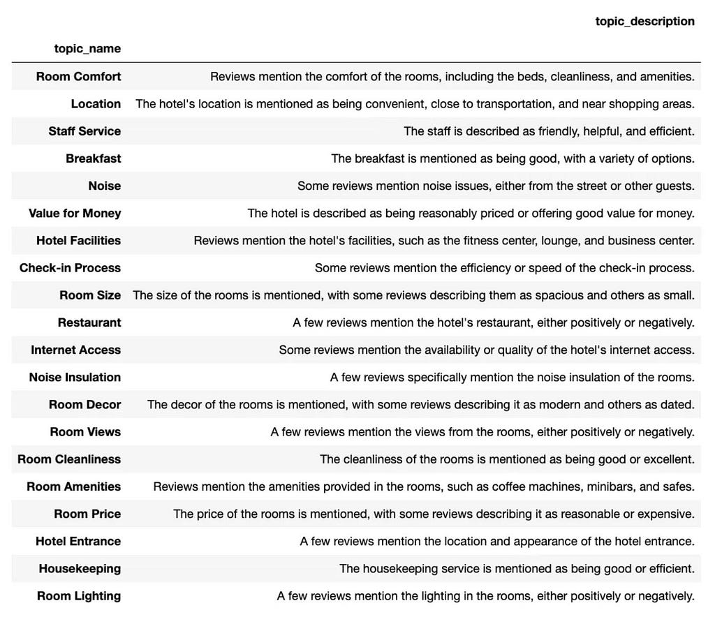
These topics can help us get a high-level overview of the customer feedback and do initial pre-filtering. But suppose we want to understand what customers think about the gym or beverages for breakfast. In that case, we will need to go through quite a lot of customer feedback ourselves from “Hotel facilities” and “Breakfast” topics.
Luckily, LLMs could help us with this analysis and save many hours of going through customers’ reviews (even though it still might be helpful to listen to the customer’s voice yourself). In this article we will discuss such approaches.
We will continue using LangChain (one of the most popular frameworks for LLM applications). You can find a basic overview of LangChain in my previous article.
Naive approaches
The most straightforward way to get comments related to a specific topic is just to look for some particular words in the texts, like “gym” or “drink”. I’ve been using this approach many times when ChatGPT didn’t exist.
The problems with this approach are pretty obvious:
- You might get quite a lot of not relevant comments about gymnasia nearby or alcoholic drinks in the hotel restaurant. Such filters are not specific enough and can’t take context into account so that you will have a lot of false positives.
- On the other hand, you might not have good enough coverage as well. People tend to use slightly different words for the same things (for example, drinks, refreshments, beverages, juices, etc). There might be typos. And this task might become even more convoluted if your customers speak different languages.
So, this approach has problems both with precision and recall. It will give you a rough understanding of the question, but its capabilities are limited.
The other potential solution is to use the same approach as with Topic Modelling: send all customer comments to LLM and ask the model to define whether they are related to our topic of interest (beverages at breakfast or gym). We can even ask the model to sum up all customer feedback and provide a conclusion.
This approach is likely to work pretty well. However, it has its limitations too: you will need to send all the documents you have to LLM each time you want to dive deeper into a particular topic. Even with high-level filtering based on topics we defined, it might be quite a lot of data to pass to LLM, and it will be rather costly.
Luckily, there is another way to solve this task, and it’s called RAG.
Retrieval-augmented generation
We have a set of documents (customer reviews), and we want to ask questions related to the content of these documents (for example, “What do customers like about breakfast?”). As we discussed before, we don’t want to send all customer reviews to LLM, so we need to have a way to define only the most relevant ones. Then, the task will be pretty straightforward: pass the user question and these documents as the context to LLM, and that’s it.
Such an approach is called Retrieval-augmented generation or RAG.

The pipeline for RAG consists of the following stages:
- Loading documents from the data sources we have.
- Splitting documents into chunks that are easy to use further.
- Storage: vector stores are often used for this use case to process data effectively.
- Retrieval of relevant to the question documents.
- Generation is passing a question and relevant documents to LLM and getting the final answer.
You might have heard that OpenAI launched Assistant API this week, which could do all these steps for you. However, I believe it’s worth going through the whole process to understand how it works and its peculiarities.
So, let’s go through all these stages step-by-step.
Loading documents
The first step is to load our documents. LangChain supports different document types, for example, CSV or JSON.
You might wonder what is the benefit of using LangChain for such basic data types. It goes without saying that you can parse CSV or JSON files using standard Python libraries. However, I recommend using LangChain data loaders API since it returns Document objects containing content and metadata. It will be easier for you to use LangChain Documents later on.
Let’s look at a bit more complex examples of data types.
We often have tasks to analyse web page content, so we have to work with HTML. Even if you’ve already mastered the BeautifulSoup library, you might find BSHTMLLoader helpful.
What’s interesting about HTML related to LLM applications is that, most likely, you will need to preprocess it a lot. If you look at any website using Browser Inspector, you will notice much more text than you see on the site. It’s used to specify the layout, formatting, styles, etc.
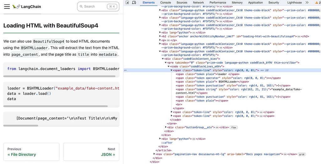
In most real-life cases, we won’t need to pass all this data to LLM. The whole HTML for a site could easily exceed 200K tokens (and only ~10–20% of it will be text you see as a user), so it would be challenging to fit it into a context size. More than that, this technical info might make the model’s job a bit harder.
So, it’s pretty standard to extract only text from HTML and use it for further analysis. To do it, you could use the command below. As a result, you will get a Document object where text from the web page is in the page_content parameter.
from langchain.document_loaders import BSHTMLLoader

loader = BSHTMLLoader("my_site.html")
data = loader.load()
The other commonly used data type is PDF. We can parse PDFs, for example, using the PyPDF library. Let’s load text from DALL-E 3 paper.
from langchain.document_loaders import PyPDFLoader
loader = PyPDFLoader("https://cdn.openai.com/papers/DALL_E_3_System_Card.pdf")
doc = loader.load()
In the output, you will get a set of Documents — one for each page. In metadata, both source and page fields will be populated.
So, as you can see, LangChain allows you to work with an extensive range of different document types.
Let’s return to our initial task. In our dataset, we have a separate .txt file with customer comments for each hotel. We need to parse all files in the directory and put them together. We can use DirectoryLoader for it.
from langchain.document_loaders import TextLoader, DirectoryLoader

text_loader_kwargs={'autodetect_encoding': True}
loader = DirectoryLoader('./hotels/london', show_progress=True,
    loader_cls=TextLoader, loader_kwargs=text_loader_kwargs)

docs = loader.load()
len(docs)
82
I’ve also used ’autodetect_encoding’: True since our texts are encoded not in standard UTF-8.
As a result, we got the list of documents — one document for each text file. We know that each document consists of individual customer reviews. It will be more effective for us to work with smaller chunks rather than with all customer comments for a hotel. So, we need to split our documents. Let’s move on to the next stage and discuss document splitting in detail.
Splitting documents
The next step is to split documents. You might wonder why we need to do this. Documents are often long and cover multiple topics, for example, Confluence pages or documentation. If we pass such lengthy texts to LLMs, we might face issues that either LLM is distracted by irrelevant information or texts don’t fit the context size.
So, to work effectively with LLMs, it’s worth defining the most relevant information from our knowledge base (set of documents) and passing only this info to the model. That’s why we need to split our documents into smaller chunks.
The most commonly used technique for general texts is recursive split by character. In LangChain, it’s implemented in RecursiveCharacterTextSplitter class.
Let’s try to understand how it works. First, you define a prioritised list of characters for the splitter (by default, it’s ["\n\n", "\n", " ", ""]). Then, the splitter goes through this list and tries to split the document by characters one by one until it gets small enough chunks. It means that this approach tries to keep semantically close parts together (paragraphs, sentences, words) until we need to split them to achieve the desired chunk size.
Let’s use the Zen of Python to see how it works. There are 824 characters, 139 words and 21 paragraphs in this text.
You can see the Zen of Python if you execute import this.
zen = '''
Beautiful is better than ugly.
Explicit is better than implicit.
Simple is better than complex.
Complex is better than complicated.
Flat is better than nested.
Sparse is better than dense.
Readability counts.
Special cases aren't special enough to break the rules.
Although practicality beats purity.
Errors should never pass silently.
Unless explicitly silenced.
In the face of ambiguity, refuse the temptation to guess.
There should be one -- and preferably only one --obvious way to do it.
Although that way may not be obvious at first unless you're Dutch.
Now is better than never.
Although never is often better than *right* now.
If the implementation is hard to explain, it's a bad idea.
If the implementation is easy to explain, it may be a good idea.
Namespaces are one honking great idea -- let's do more of those!
'''

print('Number of characters: %d' % len(zen))
print('Number of words: %d' % len(zen.replace('\n', ' ').split(' ')))
print('Number of paragraphs: %d' % len(zen.split('\n')))

# Number of characters: 825
# Number of words: 140
# Number of paragraphs: 21
Let’s use RecursiveCharacterTextSplitter and start with a relatively big chunk size equal to 300.
from langchain.text_splitter import RecursiveCharacterTextSplitter

text_splitter = RecursiveCharacterTextSplitter(
    chunk_size = 300,
    chunk_overlap  = 0,
    length_function = len,
    is_separator_regex = False,
)
text_splitter.split_text(zen)
We will get three chunks: 264, 293 and 263 characters. We could see that all sentences are held together.
All images below are made by author.

You might notice a chunk_overlap parameter that could allow you to split with overlap. It’s important because we will be passing to LLM some chunks with our questions, and it’s crucial to have enough context to make decisions based only on the information provided in each chunk.

Let’s try to add chunk_overlap.
text_splitter = RecursiveCharacterTextSplitter(
    chunk_size = 300,
    chunk_overlap  = 100,
    length_function = len,
    is_separator_regex = False,
)
text_splitter.split_text(zen)
Now, we have four splits with 264, 232, 297 and 263 characters, and we can see that our chunks overlap.

Let’s make the chunk size a bit smaller.
text_splitter = RecursiveCharacterTextSplitter(
    chunk_size = 50,
    chunk_overlap  = 10,
    length_function = len,
    is_separator_regex = False,
)
text_splitter.split_text(zen)
Now, we even had to split some longer sentences. That’s how recursive split works: since after splitting by paragraphs ("\n"), chunks are still not small enough, the splitter proceeded to " ".

You can customise the split even further. For example, you could specify length_function = lambda x: len(x.split("\n")) to use the number of paragraphs as the chunk length instead of the number of characters. It’s also quite common to split by tokens because LLMs have limited context sizes based on the number of tokens.
The other potential customisation is to use other separators to prefer to split by "," instead of " " . Let’s try to use it with a couple of sentences.
text_splitter = RecursiveCharacterTextSplitter(
    chunk_size = 50,
    chunk_overlap  = 0,
    length_function = len,
    is_separator_regex = False,
    separators=["\n\n", "\n", ", ", " ", ""]
)
text_splitter.split_text('''\
If the implementation is hard to explain, it's a bad idea.
If the implementation is easy to explain, it may be a good idea.''')
It works, but commas are not in the right places.

To fix this issue, we could use regexp with lookback as a separator.
text_splitter = RecursiveCharacterTextSplitter(
    chunk_size = 50,
    chunk_overlap  = 0,
    length_function = len,
    is_separator_regex = True,
    separators=["\n\n", "\n", "(?<=\, )", " ", ""]
)
text_splitter.split_text('''\
If the implementation is hard to explain, it's a bad idea.
If the implementation is easy to explain, it may be a good idea.''')
Now it’s fixed.

Also, LangChain provides tools for working with code so that your texts are split based on separators specific to programming languages.
However, in our case, the situation is more straightforward. We know we have individual independent comments delimited by "\n" in each file, and we just need to split by it. Unfortunately, LangChain doesn’t support such a basic use case, so we need to do a bit of hacking to make it work as we want to.
from langchain.text_splitter import CharacterTextSplitter

text_splitter = CharacterTextSplitter(
    separator = "\n",
    chunk_size = 1,
    chunk_overlap  = 0,
    length_function = lambda x: 1, # hack - usually len is used
    is_separator_regex = False
)
split_docs = text_splitter.split_documents(docs)
len(split_docs)
12890
You can find more details on why we need a hack here in my previous article about LangChain.
The significant part of the documents is metadata since it can give more context about where this chunk came from. In our case, LangChain automatically populated the source parameter for metadata so that we know which hotel each comment is related to.

There are some other approaches (i.e. for HTML or Markdown) that add titles to metadata while splitting documents. These methods could be quite helpful if you’re working with such data types.
Vector stores
Now we have comment texts and next step is to learn how to store them effectively so that we could get relevant documents for our questions.
We could store comments as strings, but it won’t help us to solve this task — we won’t be able to filter customer reviews relevant to the question.
A much more functional solution is to store documents’ embeddings.
Embeddings are high-dimensional vectors. Embeddings capture semantical meanings and relationships between words and phrases so that semantically close texts will have a smaller distance between them.
We will be using OpenAI Embeddings since they are pretty popular. OpenAI advises using the text-embedding-ada-002 model since it has better performance, more extended context and lower price. As usual, it has its risks and limitations: potential social bias and limited knowledge about recent events.
Let’s try to use Embeddings on toy examples to see how it works.
from langchain.embeddings.openai import OpenAIEmbeddings
embedding = OpenAIEmbeddings()

text1 = 'Our room (standard one) was very clean and large.'
text2 = 'Weather in London was wonderful.'
text3 = 'The room I had was actually larger than those found in other hotels in the area, and was very well appointed.'

emb1 = embedding.embed_query(text1)
emb2 = embedding.embed_query(text2)
emb3 = embedding.embed_query(text3)

print('''
Distance 1 -> 2: %.2f
Distance 1 -> 3: %.2f
Distance 2-> 3: %.2f
''' % (np.dot(emb1, emb2), np.dot(emb1, emb3), np.dot(emb2, emb3)))
We can use np.dot as cosine similarity because OpenAI embeddings are already normed.
We can see that the first and the third vectors are close to each other, while the second one differs. The first and third sentences have similar semantical meanings (they are both about the room size), while the second sentence is not close, talking about the weather. So, distances between embeddings actually reflect the semantical similarity between texts.

Now, we know how to convert comments into numeric vectors. The next question is how we should store it so that this data is easily accessible.
Let’s think about our use case. Our flow will be:
- get a question,
- calculate its embedding,
- find the most relevant document chunks related to this question (the ones with the smallest distance to this embedding),
- finally, pass found chunks to LLM as a context along with the initial question.
The regular task for the data storage will be to find K nearest vectors (K most relevant documents). So, we will need to calculate the distance (in our case, Cosine Similarity) between our question’s embedding and all the vectors we have.
Generic databases (like Snowflake or Postgres) will perform poorly for such a task. But there are databases optimised, especially for this use case — vector databases.
We will be using an open-source embedding database, Chroma. Chroma is a lightweight in-memory DB, so it’s ideal for prototyping. You can find much more options for vector stores here.
First, we need to install Chroma using pip.
pip install chromadb
We will use persist_directory to store our data locally and reload it from disk.
from langchain.vectorstores import Chroma
persist_directory = 'vector_store'

vectordb = Chroma.from_documents(
    documents=split_docs,
    embedding=embedding,
    persist_directory=persist_directory
)
To be able to load data from disk when you need it next time, execute the following command.
embedding = OpenAIEmbeddings()
vectordb = Chroma(
    persist_directory=persist_directory,
    embedding_function=embedding
)
The database initialisation might take a couple of minutes since Chroma needs to load all documents and get their embeddings using OpenAI API.
We can see that all documents have been loaded.
print(vectordb._collection.count())
12890
Now, we could use a similarity search to find top customer comments about staff politeness.
query_docs = vectordb.similarity_search('politeness of staff', k=3)
Documents look pretty relevant to the question.

We have stored our customer comments in an accessible way, and it’s time to discuss retrieval in more detail.
Retrieval
We’ve already used vectordb.similarity_search to retrieve the most related chunks to the question. In most cases, such an approach will work for you, but there could be some nuances:
- Lack of diversity — The model might return extremely close texts (even duplicates), which won’t add much new information to LLM.
- Not taking into account metadata — similarity_search doesn’t take into account the metadata information we have. For example, if I query the top-5 comments for the question “breakfast in Travelodge Farringdon”, only three comments in the result will have the source equal to uk_england_london_travelodge_london_farringdon.
- Context size limitation — as usual, we have limited LLM context size and need to fit our documents into it.
Let’s discuss techniques that could help us to solve these problems.
Addressing Diversity — MMR (Maximum Marginal Relevance)
Similarity search returns the most close responses to your question. But to provide the complete information to the model, you might want not to focus on the most similar texts. For example, for the question “breakfast in Travelodge Farringdon”, the top five customer reviews might be about coffee. If we look only at them, we will miss other comments mentioning eggs or staff behaviour and get somewhat limited view on the customer feedback.
We could use the MMR (Maximum Marginal Relevance) approach to increase the diversity of customer comments. It works pretty straightforward:
- First, we get fetch_k the most similar docs to the question using similarity_search .
- Then, we picked up k the most diverse among them.

If we want to use MMR, we should use max_marginal_relevance_search instead of similarity_search and specify fetch_k number. It’s worth keeping fetch_k relatively small so that you don’t have irrelevant answers in the output. That’s it.
query_docs = vectordb.max_marginal_relevance_search('politeness of staff',
    k = 3, fetch_k = 30)
Let’s look at the examples for the same query. We got more diverse feedback this time. There’s even a comment with negative sentiment.

Addressing specificity — LLM-aided retrieval
The other problem is that we don’t take into account the metadata while retrieving documents. To solve it, we can ask LLM to split the initial question into two parts:
- semantical filter based on document texts,
- filter based on metadata we have.
This approach is called “Self querying”.
First, let’s add a manual filter specifying a source parameter with the filename related to Travelodge Farringdon hotel.
query_docs = vectordb.similarity_search('breakfast in Travelodge Farrigdon',
  k=5,
  filter = {'source': 'hotels/london/uk_england_london_travelodge_london_farringdon'}
)
Now, let’s try to use LLM to come up with such a filter automatically. We need to describe all our metadata parameters in detail and then use SelfQueryRetriever.
from langchain.llms import OpenAI
from langchain.retrievers.self_query.base import SelfQueryRetriever
from langchain.chains.query_constructor.base import AttributeInfo

metadata_field_info = [
    AttributeInfo(
        name="source",
        description="All sources starts with 'hotels/london/uk_england_london_' \
          then goes hotel chain, constant 'london_' and location.",
        type="string",
    )
]

document_content_description = "Customer reviews for hotels"
llm = OpenAI(temperature=0.1) # low temperature to make model more factual
# by default 'text-davinci-003' is used

retriever = SelfQueryRetriever.from_llm(
    llm,
    vectordb,
    document_content_description,
    metadata_field_info,
    verbose=True
)

question = "breakfast in Travelodge Farringdon"
docs = retriever.get_relevant_documents(question, k = 5)
Our case is tricky since the source parameter in the metadata consists of multiple fields: country, city, hotel chain and location. It’s worth splitting such complex parameters into more granular ones in such situations so that the model can easily understand how to use metadata filters.
However, with a detailed prompt, it worked and returned only documents related to Travelodge Farringdon. But I must confess, it took me several iterations to achieve this result.
Let’s switch on debug and see how it works. To enter debug mode, you just need to execute the code below.
import langchain
langchain.debug = True
The complete prompt is pretty long, so let’s look at the main parts of it. Here’s the prompt’s start, which gives the model an overview of what we expect and the main criteria for the result.

Then, the few-shot prompting technique is used, and the model is provided with two examples of input and expected output. Here’s one of the examples.

We are not using a chat model like ChatGPT but general LLM (not fine-tuned on instructions). It’s trained just to predict the following tokens for the text. That’s why we finished our prompt with our question and the string Structured output: expecting the model to provide the answer.

As a result, we got from the model the initial question split into two parts: semantic one (breakfast) and metadata filters (source = hotels/london/uk_england_london_travelodge_london_farringdon)

Then, we used this logic to retrieve documents from our vector store and got only documents we need.
Addressing size limitations — Compression
The other technique for retrieval that might be handy is compression. Even though GPT 4 Turbo has a context size of 128K tokens, it’s still limited. That’s why we might want to preprocess documents and extract only relevant parts.
The main advantages are:
- You will be able to fit more documents and information into the final prompt since they will be condensed.
- You will get better, more focused results because the non-relevant context will be cleaned during preprocessing.
These benefits come with the cost — you will have more calls to LLM for compression, which means lower speed and higher price.
You can find more info about this technique in the docs.

Actually, we can even combine techniques and use MMR here. We used ContextualCompressionRetriever to get results. Also, we specified that we want just three documents in return.
from langchain.retrievers import ContextualCompressionRetriever
from langchain.retrievers.document_compressors import LLMChainExtractor

llm = OpenAI(temperature=0)
compressor = LLMChainExtractor.from_llm(llm)
compression_retriever = ContextualCompressionRetriever(
    base_compressor=compressor,
    base_retriever=vectordb.as_retriever(search_type = "mmr",
      search_kwargs={"k": 3})
)

question = "breakfast in Travelodge Farringdon"
compressed_docs = compression_retriever.get_relevant_documents(question)
As usual, understanding how it works under the hood is the most exciting part. If we look at actual calls, there are three calls to LLM to extract only relevant information from the text. Here’s an example.

In the output, we got only part of the sentence related to breakfast, so compression helps.

There are many more beneficial approaches for retrieval, for example, techniques from classic NLP: SVM or TF-IDF. Different retrievers might be helpful in different situations, so I recommend you compare different versions for your task and select the most suitable one for your use case.
Generation
Finally, we got to the last stage: we will combine everything and generate the final answer.
Here’s a scheme on how it all will work:
- we get a question from a user,
- we retrieve relevant documents for this question from the vector store using embeddings,
- we pass the initial question along with retrieved documents to the LLM and get the final answer.

In LangChain, we could use RetrievalQA chain to implement this flow quickly.
from langchain.chains import RetrievalQA

from langchain.chat_models import ChatOpenAI
llm = ChatOpenAI(model_name='gpt-4', temperature=0.1)

qa_chain = RetrievalQA.from_chain_type(
    llm,
    retriever=vectordb.as_retriever(search_kwargs={"k": 3})
)

result = qa_chain({"query": "what customers like about staff in the hotel?"})
Let’s look at the call to ChatGPT. As you can see, we passed retrieved documents along with the user query.

Here’s an output from the model.

We can tweak the model’s behaviour, customising prompt. For example, we could ask the model to be more concise.
from langchain.prompts import PromptTemplate

template = """
Use the following pieces of context to answer the question at the end.
If you don't know the answer, just say that you don't know, don't try
to make up an answer.
Keep the answer as concise as possible. Use 1 sentence to sum all points up.
______________
{context}
Question: {question}
Helpful Answer:"""

QA_CHAIN_PROMPT = PromptTemplate.from_template(template)

qa_chain = RetrievalQA.from_chain_type(
    llm,
    retriever=vectordb.as_retriever(),
    return_source_documents=True,
    chain_type_kwargs={"prompt": QA_CHAIN_PROMPT}
)
result = qa_chain({"query": "what customers like about staff in the hotel?"})
We got a much shorter answer this time. Also, since we specified return_source_documents=True, we got a set of documents in return. It could be helpful for debugging.

As we’ve seen, all retrieved documents are combined in one prompt by default. This approach is excellent and straightforward since it invokes only one call to LLM. The only limitation is that your documents must fit the context size. If they don’t, you need to apply more complex techniques.
Let’s look at different chain types that could allow us to work with any number of documents. The first one is MapReduce.
This approach is similar to classical MapReduce: we generate answers based on each retrieved document (map stage) and then combine these answers into the final one (reduce stage).

The limitations of all such approaches are cost and speed. Instead of one call to LLM, you need to do a call for each retrieved document.
Regarding code, we just need to specify chain_type="map_reduce" to change behaviour.
qa_chain_mr = RetrievalQA.from_chain_type(
    llm,
    retriever=vectordb.as_retriever(),
    chain_type="map_reduce"
)
result = qa_chain_mr({"query": "what customers like about staff in the hotel?"})
In the result, we got the following output.

Let’s see how it works using debug mode. Since it’s a MapReduce, we first sent each document to LLM and got the answer based on this chunk. Here’s an example of prompt for one of the chunks.

Then, we combine all the results and ask LLM to come up with the final answer.

That’s it.
There is another drawback specific to the MapReduce approach. The model sees each document separately and doesn’t have them all in the same context, which might lead to worse results.
We can overcome this drawback with the Refine chain type. Then, we will look at documents sequentially and allow the model to refine the answer on each iteration.

Again, we just need to change chain_type to test another approach.
qa_chain_refine = RetrievalQA.from_chain_type(
    llm,
    retriever=vectordb.as_retriever(),
    chain_type="refine"
)
result = qa_chain_refine({"query": "what customers like about staff in the hotel?"})
With the Refine chain, we got a bit more wordy and complete answer.

Let’s see how it works using debug. For the first chunk, we are starting from scratch.

Then, we pass the current answer and a new chunk and give the model a chance to refine its answer.

Then, we repeat the refining prompt for each remaining retrieved document and get the final result.
That’s all that I wanted to tell you today. Let’s do a quick recap.
Summary
In this article, we went through the whole process of Retrieval-augmented generation:
- We’ve looked at different data loaders.
- We’ve discussed possible approaches to data splitting and their potential nuances.
- We’ve learned what embeddings are and set up a vector store to access data effectively.
- We’ve found different solutions for retrieval issues and learned how to increase diversity, to overcome context size limitations and to use metadata.
- Finally, we’ve used the RetrievalQA chain to generate the answer based on our data and compared different chain types.
This knowledge should be enough for start building something similar with your data.
Thank you a lot for reading this article. I hope it was insightful to you. If you have any follow-up questions or comments, please leave them in the comments section.
Dataset
Ganesan, Kavita and Zhai, ChengXiang. (2011). OpinRank Review Dataset.
UCI Machine Learning Repository (CC BY 4.0). https://doi.org/10.24432/C5QW4W
Reference
This article is based on information from the courses:
- “LangChain for LLM Application Development” by DeepLearning.AI and LangChain,
- “LangChain: Chat with your data” by DeepLearning.AI and LangChain.
RAG: How to Talk to Your Data was originally published in Towards Data Science on Medium, where people are continuing the conversation by highlighting and responding to this story.
Comprehensive guide on how to analyse customer feedback using ChatGPT

In my previous articles, we discussed how to do Topic Modelling using ChatGPT. Our task was to analyse customer comments for different hotel chains and identify the main topics mentioned for each hotel.
As a result of such Topic Modelling, we know topics for each customer review and can easily filter by them and dive deeper. However, in real life, it’s impossible to have such an exhaustive set of topics that could cover all your possible use cases.
For example, here’s the list of topics we identified from customer feedback earlier.
These topics can help us get a high-level overview of the customer feedback and do initial pre-filtering. But suppose we want to understand what customers think about the gym or beverages for breakfast. In that case, we will need to go through quite a lot of customer feedback ourselves from “Hotel facilities” and “Breakfast” topics.
Luckily, LLMs could help us with this analysis and save many hours of going through customers’ reviews (even though it still might be helpful to listen to the customer’s voice yourself). In this article we will discuss such approaches.
We will continue using LangChain (one of the most popular frameworks for LLM applications). You can find a basic overview of LangChain in my previous article.
Naive approaches
The most straightforward way to get comments related to a specific topic is just to look for some particular words in the texts, like “gym” or “drink”. I’ve been using this approach many times when ChatGPT didn’t exist.
The problems with this approach are pretty obvious:
- You might get quite a lot of not relevant comments about gymnasia nearby or alcoholic drinks in the hotel restaurant. Such filters are not specific enough and can’t take context into account so that you will have a lot of false positives.
- On the other hand, you might not have good enough coverage as well. People tend to use slightly different words for the same things (for example, drinks, refreshments, beverages, juices, etc). There might be typos. And this task might become even more convoluted if your customers speak different languages.
So, this approach has problems both with precision and recall. It will give you a rough understanding of the question, but its capabilities are limited.
The other potential solution is to use the same approach as with Topic Modelling: send all customer comments to LLM and ask the model to define whether they are related to our topic of interest (beverages at breakfast or gym). We can even ask the model to sum up all customer feedback and provide a conclusion.
This approach is likely to work pretty well. However, it has its limitations too: you will need to send all the documents you have to LLM each time you want to dive deeper into a particular topic. Even with high-level filtering based on topics we defined, it might be quite a lot of data to pass to LLM, and it will be rather costly.
Luckily, there is another way to solve this task, and it’s called RAG.
Retrieval-augmented generation
We have a set of documents (customer reviews), and we want to ask questions related to the content of these documents (for example, “What do customers like about breakfast?”). As we discussed before, we don’t want to send all customer reviews to LLM, so we need to have a way to define only the most relevant ones. Then, the task will be pretty straightforward: pass the user question and these documents as the context to LLM, and that’s it.
Such an approach is called Retrieval-augmented generation or RAG.
The pipeline for RAG consists of the following stages:
- Loading documents from the data sources we have.
- Splitting documents into chunks that are easy to use further.
- Storage: vector stores are often used for this use case to process data effectively.
- Retrieval of relevant to the question documents.
- Generation is passing a question and relevant documents to LLM and getting the final answer.
You might have heard that OpenAI launched Assistant API this week, which could do all these steps for you. However, I believe it’s worth going through the whole process to understand how it works and its peculiarities.
So, let’s go through all these stages step-by-step.
Loading documents
The first step is to load our documents. LangChain supports different document types, for example, CSV or JSON.
You might wonder what is the benefit of using LangChain for such basic data types. It goes without saying that you can parse CSV or JSON files using standard Python libraries. However, I recommend using LangChain data loaders API since it returns Document objects containing content and metadata. It will be easier for you to use LangChain Documents later on.
Let’s look at a bit more complex examples of data types.
We often have tasks to analyse web page content, so we have to work with HTML. Even if you’ve already mastered the BeautifulSoup library, you might find BSHTMLLoader helpful.
What’s interesting about HTML related to LLM applications is that, most likely, you will need to preprocess it a lot. If you look at any website using Browser Inspector, you will notice much more text than you see on the site. It’s used to specify the layout, formatting, styles, etc.
In most real-life cases, we won’t need to pass all this data to LLM. The whole HTML for a site could easily exceed 200K tokens (and only ~10–20% of it will be text you see as a user), so it would be challenging to fit it into a context size. More than that, this technical info might make the model’s job a bit harder.
So, it’s pretty standard to extract only text from HTML and use it for further analysis. To do it, you could use the command below. As a result, you will get a Document object where text from the web page is in the page_content parameter.
from langchain.document_loaders import BSHTMLLoader

loader = BSHTMLLoader("my_site.html")
data = loader.load()
The other commonly used data type is PDF. We can parse PDFs, for example, using the PyPDF library. Let’s load text from DALL-E 3 paper.
from langchain.document_loaders import PyPDFLoader
loader = PyPDFLoader("https://cdn.openai.com/papers/DALL_E_3_System_Card.pdf")
doc = loader.load()
In the output, you will get a set of Documents — one for each page. In metadata, both source and page fields will be populated.
So, as you can see, LangChain allows you to work with an extensive range of different document types.
Let’s return to our initial task. In our dataset, we have a separate .txt file with customer comments for each hotel. We need to parse all files in the directory and put them together. We can use DirectoryLoader for it.
from langchain.document_loaders import TextLoader, DirectoryLoader

text_loader_kwargs={'autodetect_encoding': True}
loader = DirectoryLoader('./hotels/london', show_progress=True,
    loader_cls=TextLoader, loader_kwargs=text_loader_kwargs)

docs = loader.load()
len(docs)
82
I’ve also used ’autodetect_encoding’: True since our texts are encoded not in standard UTF-8.
As a result, we got the list of documents — one document for each text file. We know that each document consists of individual customer reviews. It will be more effective for us to work with smaller chunks rather than with all customer comments for a hotel. So, we need to split our documents. Let’s move on to the next stage and discuss document splitting in detail.
Splitting documents
The next step is to split documents. You might wonder why we need to do this. Documents are often long and cover multiple topics, for example, Confluence pages or documentation. If we pass such lengthy texts to LLMs, we might face issues that either LLM is distracted by irrelevant information or texts don’t fit the context size.
So, to work effectively with LLMs, it’s worth defining the most relevant information from our knowledge base (set of documents) and passing only this info to the model. That’s why we need to split our documents into smaller chunks.
The most commonly used technique for general texts is recursive split by character. In LangChain, it’s implemented in RecursiveCharacterTextSplitter class.
Let’s try to understand how it works. First, you define a prioritised list of characters for the splitter (by default, it’s ["\n\n", "\n", " ", ""]). Then, the splitter goes through this list and tries to split the document by characters one by one until it gets small enough chunks. It means that this approach tries to keep semantically close parts together (paragraphs, sentences, words) until we need to split them to achieve the desired chunk size.
Let’s use the Zen of Python to see how it works. There are 824 characters, 139 words and 21 paragraphs in this text.
You can see the Zen of Python if you execute import this.
zen = '''
Beautiful is better than ugly.
Explicit is better than implicit.
Simple is better than complex.
Complex is better than complicated.
Flat is better than nested.
Sparse is better than dense.
Readability counts.
Special cases aren't special enough to break the rules.
Although practicality beats purity.
Errors should never pass silently.
Unless explicitly silenced.
In the face of ambiguity, refuse the temptation to guess.
There should be one -- and preferably only one --obvious way to do it.
Although that way may not be obvious at first unless you're Dutch.
Now is better than never.
Although never is often better than *right* now.
If the implementation is hard to explain, it's a bad idea.
If the implementation is easy to explain, it may be a good idea.
Namespaces are one honking great idea -- let's do more of those!
'''

print('Number of characters: %d' % len(zen))
print('Number of words: %d' % len(zen.replace('\n', ' ').split(' ')))
print('Number of paragraphs: %d' % len(zen.split('\n')))

# Number of characters: 825
# Number of words: 140
# Number of paragraphs: 21
Let’s use RecursiveCharacterTextSplitter and start with a relatively big chunk size equal to 300.
from langchain.text_splitter import RecursiveCharacterTextSplitter

text_splitter = RecursiveCharacterTextSplitter(
    chunk_size = 300,
    chunk_overlap  = 0,
    length_function = len,
    is_separator_regex = False,
)
text_splitter.split_text(zen)
We will get three chunks: 264, 293 and 263 characters. We could see that all sentences are held together.
All images below are made by author.
You might notice a chunk_overlap parameter that could allow you to split with overlap. It’s important because we will be passing to LLM some chunks with our questions, and it’s crucial to have enough context to make decisions based only on the information provided in each chunk.
Let’s try to add chunk_overlap.
text_splitter = RecursiveCharacterTextSplitter(
    chunk_size = 300,
    chunk_overlap  = 100,
    length_function = len,
    is_separator_regex = False,
)
text_splitter.split_text(zen)
Now, we have four splits with 264, 232, 297 and 263 characters, and we can see that our chunks overlap.
Let’s make the chunk size a bit smaller.
text_splitter = RecursiveCharacterTextSplitter(
    chunk_size = 50,
    chunk_overlap  = 10,
    length_function = len,
    is_separator_regex = False,
)
text_splitter.split_text(zen)
Now, we even had to split some longer sentences. That’s how recursive split works: since after splitting by paragraphs ("\n"), chunks are still not small enough, the splitter proceeded to " ".
You can customise the split even further. For example, you could specify length_function = lambda x: len(x.split("\n")) to use the number of paragraphs as the chunk length instead of the number of characters. It’s also quite common to split by tokens because LLMs have limited context sizes based on the number of tokens.
The other potential customisation is to use other separators to prefer to split by "," instead of " " . Let’s try to use it with a couple of sentences.
text_splitter = RecursiveCharacterTextSplitter(
    chunk_size = 50,
    chunk_overlap  = 0,
    length_function = len,
    is_separator_regex = False,
    separators=["\n\n", "\n", ", ", " ", ""]
)
text_splitter.split_text('''\
If the implementation is hard to explain, it's a bad idea.
If the implementation is easy to explain, it may be a good idea.''')
It works, but commas are not in the right places.
To fix this issue, we could use regexp with lookback as a separator.
text_splitter = RecursiveCharacterTextSplitter(
    chunk_size = 50,
    chunk_overlap  = 0,
    length_function = len,
    is_separator_regex = True,
    separators=["\n\n", "\n", "(?<=\, )", " ", ""]
)
text_splitter.split_text('''\
If the implementation is hard to explain, it's a bad idea.
If the implementation is easy to explain, it may be a good idea.''')
Now it’s fixed.
Also, LangChain provides tools for working with code so that your texts are split based on separators specific to programming languages.
However, in our case, the situation is more straightforward. We know we have individual independent comments delimited by "\n" in each file, and we just need to split by it. Unfortunately, LangChain doesn’t support such a basic use case, so we need to do a bit of hacking to make it work as we want to.
from langchain.text_splitter import CharacterTextSplitter

text_splitter = CharacterTextSplitter(
    separator = "\n",
    chunk_size = 1,
    chunk_overlap  = 0,
    length_function = lambda x: 1, # hack - usually len is used
    is_separator_regex = False
)
split_docs = text_splitter.split_documents(docs)
len(split_docs)
12890
You can find more details on why we need a hack here in my previous article about LangChain.
The significant part of the documents is metadata since it can give more context about where this chunk came from. In our case, LangChain automatically populated the source parameter for metadata so that we know which hotel each comment is related to.
There are some other approaches (i.e. for HTML or Markdown) that add titles to metadata while splitting documents. These methods could be quite helpful if you’re working with such data types.
Vector stores
Now we have comment texts and next step is to learn how to store them effectively so that we could get relevant documents for our questions.
We could store comments as strings, but it won’t help us to solve this task — we won’t be able to filter customer reviews relevant to the question.
A much more functional solution is to store documents’ embeddings.
Embeddings are high-dimensional vectors. Embeddings capture semantical meanings and relationships between words and phrases so that semantically close texts will have a smaller distance between them.
We will be using OpenAI Embeddings since they are pretty popular. OpenAI advises using the text-embedding-ada-002 model since it has better performance, more extended context and lower price. As usual, it has its risks and limitations: potential social bias and limited knowledge about recent events.
Let’s try to use Embeddings on toy examples to see how it works.
from langchain.embeddings.openai import OpenAIEmbeddings
embedding = OpenAIEmbeddings()

text1 = 'Our room (standard one) was very clean and large.'
text2 = 'Weather in London was wonderful.'
text3 = 'The room I had was actually larger than those found in other hotels in the area, and was very well appointed.'

emb1 = embedding.embed_query(text1)
emb2 = embedding.embed_query(text2)
emb3 = embedding.embed_query(text3)

print('''
Distance 1 -> 2: %.2f
Distance 1 -> 3: %.2f
Distance 2-> 3: %.2f
''' % (np.dot(emb1, emb2), np.dot(emb1, emb3), np.dot(emb2, emb3)))
We can use np.dot as cosine similarity because OpenAI embeddings are already normed.
We can see that the first and the third vectors are close to each other, while the second one differs. The first and third sentences have similar semantical meanings (they are both about the room size), while the second sentence is not close, talking about the weather. So, distances between embeddings actually reflect the semantical similarity between texts.
Now, we know how to convert comments into numeric vectors. The next question is how we should store it so that this data is easily accessible.
Let’s think about our use case. Our flow will be:
- get a question,
- calculate its embedding,
- find the most relevant document chunks related to this question (the ones with the smallest distance to this embedding),
- finally, pass found chunks to LLM as a context along with the initial question.
The regular task for the data storage will be to find K nearest vectors (K most relevant documents). So, we will need to calculate the distance (in our case, Cosine Similarity) between our question’s embedding and all the vectors we have.
Generic databases (like Snowflake or Postgres) will perform poorly for such a task. But there are databases optimised, especially for this use case — vector databases.
We will be using an open-source embedding database, Chroma. Chroma is a lightweight in-memory DB, so it’s ideal for prototyping. You can find much more options for vector stores here.
First, we need to install Chroma using pip.
pip install chromadb
We will use persist_directory to store our data locally and reload it from disk.
from langchain.vectorstores import Chroma
persist_directory = 'vector_store'

vectordb = Chroma.from_documents(
    documents=split_docs,
    embedding=embedding,
    persist_directory=persist_directory
)
To be able to load data from disk when you need it next time, execute the following command.
embedding = OpenAIEmbeddings()
vectordb = Chroma(
    persist_directory=persist_directory,
    embedding_function=embedding
)
The database initialisation might take a couple of minutes since Chroma needs to load all documents and get their embeddings using OpenAI API.
We can see that all documents have been loaded.
print(vectordb._collection.count())
12890
Now, we could use a similarity search to find top customer comments about staff politeness.
query_docs = vectordb.similarity_search('politeness of staff', k=3)
Documents look pretty relevant to the question.
We have stored our customer comments in an accessible way, and it’s time to discuss retrieval in more detail.
Retrieval
We’ve already used vectordb.similarity_search to retrieve the most related chunks to the question. In most cases, such an approach will work for you, but there could be some nuances:
- Lack of diversity — The model might return extremely close texts (even duplicates), which won’t add much new information to LLM.
- Not taking into account metadata — similarity_search doesn’t take into account the metadata information we have. For example, if I query the top-5 comments for the question “breakfast in Travelodge Farringdon”, only three comments in the result will have the source equal to uk_england_london_travelodge_london_farringdon.
- Context size limitation — as usual, we have limited LLM context size and need to fit our documents into it.
Let’s discuss techniques that could help us to solve these problems.
Addressing Diversity — MMR (Maximum Marginal Relevance)
Similarity search returns the most close responses to your question. But to provide the complete information to the model, you might want not to focus on the most similar texts. For example, for the question “breakfast in Travelodge Farringdon”, the top five customer reviews might be about coffee. If we look only at them, we will miss other comments mentioning eggs or staff behaviour and get somewhat limited view on the customer feedback.
We could use the MMR (Maximum Marginal Relevance) approach to increase the diversity of customer comments. It works pretty straightforward:
- First, we get fetch_k the most similar docs to the question using similarity_search .
- Then, we picked up k the most diverse among them.
If we want to use MMR, we should use max_marginal_relevance_search instead of similarity_search and specify fetch_k number. It’s worth keeping fetch_k relatively small so that you don’t have irrelevant answers in the output. That’s it.
query_docs = vectordb.max_marginal_relevance_search('politeness of staff',
    k = 3, fetch_k = 30)
Let’s look at the examples for the same query. We got more diverse feedback this time. There’s even a comment with negative sentiment.
Addressing specificity — LLM-aided retrieval
The other problem is that we don’t take into account the metadata while retrieving documents. To solve it, we can ask LLM to split the initial question into two parts:
- semantical filter based on document texts,
- filter based on metadata we have.
This approach is called “Self querying”.
First, let’s add a manual filter specifying a source parameter with the filename related to Travelodge Farringdon hotel.
query_docs = vectordb.similarity_search('breakfast in Travelodge Farrigdon',
  k=5,
  filter = {'source': 'hotels/london/uk_england_london_travelodge_london_farringdon'}
)
Now, let’s try to use LLM to come up with such a filter automatically. We need to describe all our metadata parameters in detail and then use SelfQueryRetriever.
from langchain.llms import OpenAI
from langchain.retrievers.self_query.base import SelfQueryRetriever
from langchain.chains.query_constructor.base import AttributeInfo

metadata_field_info = [
    AttributeInfo(
        name="source",
        description="All sources starts with 'hotels/london/uk_england_london_' \
          then goes hotel chain, constant 'london_' and location.",
        type="string",
    )
]

document_content_description = "Customer reviews for hotels"
llm = OpenAI(temperature=0.1) # low temperature to make model more factual
# by default 'text-davinci-003' is used

retriever = SelfQueryRetriever.from_llm(
    llm,
    vectordb,
    document_content_description,
    metadata_field_info,
    verbose=True
)

question = "breakfast in Travelodge Farringdon"
docs = retriever.get_relevant_documents(question, k = 5)
Our case is tricky since the source parameter in the metadata consists of multiple fields: country, city, hotel chain and location. It’s worth splitting such complex parameters into more granular ones in such situations so that the model can easily understand how to use metadata filters.
However, with a detailed prompt, it worked and returned only documents related to Travelodge Farringdon. But I must confess, it took me several iterations to achieve this result.
Let’s switch on debug and see how it works. To enter debug mode, you just need to execute the code below.
import langchain
langchain.debug = True
The complete prompt is pretty long, so let’s look at the main parts of it. Here’s the prompt’s start, which gives the model an overview of what we expect and the main criteria for the result.
Then, the few-shot prompting technique is used, and the model is provided with two examples of input and expected output. Here’s one of the examples.
We are not using a chat model like ChatGPT but general LLM (not fine-tuned on instructions). It’s trained just to predict the following tokens for the text. That’s why we finished our prompt with our question and the string Structured output: expecting the model to provide the answer.
As a result, we got from the model the initial question split into two parts: semantic one (breakfast) and metadata filters (source = hotels/london/uk_england_london_travelodge_london_farringdon)
Then, we used this logic to retrieve documents from our vector store and got only documents we need.
Addressing size limitations — Compression
The other technique for retrieval that might be handy is compression. Even though GPT 4 Turbo has a context size of 128K tokens, it’s still limited. That’s why we might want to preprocess documents and extract only relevant parts.
The main advantages are:
- You will be able to fit more documents and information into the final prompt since they will be condensed.
- You will get better, more focused results because the non-relevant context will be cleaned during preprocessing.
These benefits come with the cost — you will have more calls to LLM for compression, which means lower speed and higher price.
You can find more info about this technique in the docs.
Actually, we can even combine techniques and use MMR here. We used ContextualCompressionRetriever to get results. Also, we specified that we want just three documents in return.
from langchain.retrievers import ContextualCompressionRetriever
from langchain.retrievers.document_compressors import LLMChainExtractor

llm = OpenAI(temperature=0)
compressor = LLMChainExtractor.from_llm(llm)
compression_retriever = ContextualCompressionRetriever(
    base_compressor=compressor,
    base_retriever=vectordb.as_retriever(search_type = "mmr",
      search_kwargs={"k": 3})
)

question = "breakfast in Travelodge Farringdon"
compressed_docs = compression_retriever.get_relevant_documents(question)
As usual, understanding how it works under the hood is the most exciting part. If we look at actual calls, there are three calls to LLM to extract only relevant information from the text. Here’s an example.
In the output, we got only part of the sentence related to breakfast, so compression helps.
There are many more beneficial approaches for retrieval, for example, techniques from classic NLP: SVM or TF-IDF. Different retrievers might be helpful in different situations, so I recommend you compare different versions for your task and select the most suitable one for your use case.
Generation
Finally, we got to the last stage: we will combine everything and generate the final answer.
Here’s a scheme on how it all will work:
- we get a question from a user,
- we retrieve relevant documents for this question from the vector store using embeddings,
- we pass the initial question along with retrieved documents to the LLM and get the final answer.
In LangChain, we could use RetrievalQA chain to implement this flow quickly.
from langchain.chains import RetrievalQA

from langchain.chat_models import ChatOpenAI
llm = ChatOpenAI(model_name='gpt-4', temperature=0.1)

qa_chain = RetrievalQA.from_chain_type(
    llm,
    retriever=vectordb.as_retriever(search_kwargs={"k": 3})
)

result = qa_chain({"query": "what customers like about staff in the hotel?"})
Let’s look at the call to ChatGPT. As you can see, we passed retrieved documents along with the user query.
Here’s an output from the model.
We can tweak the model’s behaviour, customising prompt. For example, we could ask the model to be more concise.
from langchain.prompts import PromptTemplate

template = """
Use the following pieces of context to answer the question at the end.
If you don't know the answer, just say that you don't know, don't try
to make up an answer.
Keep the answer as concise as possible. Use 1 sentence to sum all points up.
______________
{context}
Question: {question}
Helpful Answer:"""

QA_CHAIN_PROMPT = PromptTemplate.from_template(template)

qa_chain = RetrievalQA.from_chain_type(
    llm,
    retriever=vectordb.as_retriever(),
    return_source_documents=True,
    chain_type_kwargs={"prompt": QA_CHAIN_PROMPT}
)
result = qa_chain({"query": "what customers like about staff in the hotel?"})
We got a much shorter answer this time. Also, since we specified return_source_documents=True, we got a set of documents in return. It could be helpful for debugging.
As we’ve seen, all retrieved documents are combined in one prompt by default. This approach is excellent and straightforward since it invokes only one call to LLM. The only limitation is that your documents must fit the context size. If they don’t, you need to apply more complex techniques.
Let’s look at different chain types that could allow us to work with any number of documents. The first one is MapReduce.
This approach is similar to classical MapReduce: we generate answers based on each retrieved document (map stage) and then combine these answers into the final one (reduce stage).
The limitations of all such approaches are cost and speed. Instead of one call to LLM, you need to do a call for each retrieved document.
Regarding code, we just need to specify chain_type="map_reduce" to change behaviour.
qa_chain_mr = RetrievalQA.from_chain_type(
    llm,
    retriever=vectordb.as_retriever(),
    chain_type="map_reduce"
)
result = qa_chain_mr({"query": "what customers like about staff in the hotel?"})
In the result, we got the following output.
Let’s see how it works using debug mode. Since it’s a MapReduce, we first sent each document to LLM and got the answer based on this chunk. Here’s an example of prompt for one of the chunks.
Then, we combine all the results and ask LLM to come up with the final answer.
That’s it.
There is another drawback specific to the MapReduce approach. The model sees each document separately and doesn’t have them all in the same context, which might lead to worse results.
We can overcome this drawback with the Refine chain type. Then, we will look at documents sequentially and allow the model to refine the answer on each iteration.
Again, we just need to change chain_type to test another approach.
qa_chain_refine = RetrievalQA.from_chain_type(
    llm,
    retriever=vectordb.as_retriever(),
    chain_type="refine"
)
result = qa_chain_refine({"query": "what customers like about staff in the hotel?"})
With the Refine chain, we got a bit more wordy and complete answer.
Let’s see how it works using debug. For the first chunk, we are starting from scratch.
Then, we pass the current answer and a new chunk and give the model a chance to refine its answer.
Then, we repeat the refining prompt for each remaining retrieved document and get the final result.
That’s all that I wanted to tell you today. Let’s do a quick recap.
Summary
In this article, we went through the whole process of Retrieval-augmented generation:
- We’ve looked at different data loaders.
- We’ve discussed possible approaches to data splitting and their potential nuances.
- We’ve learned what embeddings are and set up a vector store to access data effectively.
- We’ve found different solutions for retrieval issues and learned how to increase diversity, to overcome context size limitations and to use metadata.
- Finally, we’ve used the RetrievalQA chain to generate the answer based on our data and compared different chain types.
This knowledge should be enough for start building something similar with your data.
Thank you a lot for reading this article. I hope it was insightful to you. If you have any follow-up questions or comments, please leave them in the comments section.
Dataset
Ganesan, Kavita and Zhai, ChengXiang. (2011). OpinRank Review Dataset.
UCI Machine Learning Repository (CC BY 4.0). https://doi.org/10.24432/C5QW4W
Reference
This article is based on information from the courses:
- “LangChain for LLM Application Development” by DeepLearning.AI and LangChain,
- “LangChain: Chat with your data” by DeepLearning.AI and LangChain.
RAG: How to Talk to Your Data was originally published in Towards Data Science on Medium, where people are continuing the conversation by highlighting and responding to this story.
Denial of responsibility! Techno Blender is an automatic aggregator of the all world’s media. In each content, the hyperlink to the primary source is specified. All trademarks belong to their rightful owners, all materials to their authors. If you are the owner of the content and do not want us to publish your materials, please contact us by email – [email protected]. The content will be deleted within 24 hours.