
Scene Graph Generation and its Application in Robotics
Let’s have a small talk about visualizing images with interactive graphical representation!
Scene graph generation is the process of generating scene graphs and a scene graph contains the visual understanding of an image in the form of a graph. It has nodes and edges representing the objects and their relationships, respectively. Contextual information about the scenes can help in semantic scene understanding. Although there are certain challenges such as uncertainty of real-world scenarios or unavailability of a standard dataset, researchers are trying to apply the scene graphs in the field of robotics. This write-up contains two major parts: one is about how scene graphs can be obtained by having an in-depth discussion about two state-of-the-art approaches for scene graph generation based on region-based convolutional neural networks, and the other part deals with the application of scene graphs in robot planning. In its former part, this article further explains that only having a numerical metric for model evaluation is insufficient for proper performance analysis. The latter part includes a thorough explanation of a method that uses the concept of scene graphs for visual context-aware robot planning.
1. Introduction
When considering the description of image elements in words, well-known active techniques such as image segmentation, object classification, activity identification, etc. play a significant role in the process. Scene Graph Generation (SGG) is a method to generate scene graphs (SGs), by depicting objects (e.g., humans, animals, etc.) and their attributes (e.g., color, clothes, vehicles, etc.) as nodes, and the relationships among objects as the edges. Fig. 1a and 1b shows how a scene graph generated from an RGB image usually looks like. It can be seen that the distinct colored nodes depict different major objects in the image (a male, a female, and a vehicle), the information about these objects is shown by the nodes having the variant of the same node color, and the edges are labeled with verbs showing a connection, or we can say relation among the nodes. The research has been going on for past years to make the SGs possible even for small details in the image.
This article extensively discusses two approaches in the upcoming sections for a better understanding of generating scene graphs. The write-up structure comprises six sections. The brief start of SGG and its prior applications including image and video captioning is explained in section 2. Section 3 describes the state-of-the-art methods with their model description. The experimental analysis of these methods is discussed and compared in section 4. Section 5 discusses some possible applications of SGs in the field of robotics with a main focus on robot planning, and also how having accurate SGs will make applications like telepresence robots, human-robot collaboration, etc. much easier to implement. Finally, section 6 concludes the entire literature.
2. Related Work
The SGs have a history of distinct applications, for instance, image and video captioning, visual question answering, 3D scene understanding, many applications in robotics, etc. [10] [3]. Most of the recent approaches include machine learning methods like Region-based Convolutional Neural Networks (R-CNN) [8], faster R-CNN [9], Recurrent Neural Networks (RNN) [7], etc. [7] proposed a structure that takes the image as input, then passes messages containing contextual information, and refines the prediction using RNN. Another method [6] uses the energy model of the image to generate comprehensive scene graphs. The datasets for SGG are also obtained using different real-world scenarios, images, and videos. The dataset mentioned here is a subset [7] of Visual Genome [4] containing 108,073 human-annotated images.
3. State-of-the-Art Approaches
3.1 Graph R-CNN Approach
J. Yang et. al. [8] proposes a model that first considers all the objects connected by an edge, relationship, then nullifies the unlikely relationship using a parameter called relatedness. For instance, it is more likely to have a relation between car and wheel, than a building and a wheel.
The paper shows a novel framework, namely Graph R-CNN with the introduction of a new evaluation metric, SGGen+. The model consists of three blocks, first to extract object nodes, second to remove unlikely edges, and finally to propagate graph context throughout the remaining graph so that the final scene graph can be produced. The novelty resides in the second and third block of the model, having a new relation proposal network (RePN) which computes relatedness that further helps in removing unlikely relationships, also called relation edge pruning and an attentional graph convolutional network (aGCN) that constitutes the propagation of higher-order context that leads to an update in scene graph giving it a final touch, respectively. Basically, the final block labeled the generated scene graph. The probability distribution of the whole idea can be depicted by the equation below, where for image I, O is the set of objects, R is the relation among objects, and Rl and Ol are relation and object labels respectively.
Pr(G|I) = Pr(O|I) * Pr(R|O, I) * Pr(Rl, Ol|O, R, I)
Fig. 2 shows the entire algorithm in pictorial form, and how all three stages work consecutively. The pipeline can be described as: using faster R-CNN for object detection, then generating an initial graph with all defined relationships, then pruning unlikely edges based on relatedness score, and then finally using aGCN for refining.
3.2 Stacked Motif Network (MotifNet)
R. Zellers et. al. [9] proposes a network that performs bounding box collection, object identification, and relation identification consecutively. The method shows the intense use of faster R-CNN and Long Short-term Memory (LSTM) networks. In contrast with Graph R-CNN, this method is based on detecting the relationships among objects and adding the relationship edges.
The idea here can be seen as a conditional probability equation, as shown in the equation below, which states the probability to find graph G of image I is given as the product of the probability of finding bounding box array B given I, probability of obtaining object O given B and I, and the probability of getting relations R among O given B, O and I.
Pr(G|I) = Pr(B|I) * Pr(O|B,I) * Pr(R|B,O,I)
Firstly, to find the set of the bounding box, they also use faster R-CNN, as in [8], shown on the left side of Fig. 3. It uses the VGG backbone structure for object identification while determining bounding boxes in I. Then, the model proceeds further with bidirectional LSTM layers depicted by the object context layer in Fig. 3. This block of layers generates the object labels for each bounding box region, bi ∈ B. Another bidirectional LSTM layers block is again used for determining relations as edge context, portrayed in the same figure. The output is computed as determining the edge labels which clearly depict the outer product with objects and relations among them. The detailed model structure can be learned in [9].
4. Experiments in State-of-the-Art Approaches
4.1 Experimental Setup
The setup for both methods is described below:
Graph R-CNN: The use of faster R-CNN with VGG16 backbone to ensure object detection is implemented via PyTorch. For the RePN implementation, a multi-layer perceptron structure is used to analyze the relatedness score using two projection functions, each for subject and object relation. Two aGCN layers are used, one for the feature level, the result of which is sent to the other one at the semantic level. The training is done in two stages, first only the object detector is trained, and then the whole model is trained jointly.
MotifNet: The images that are fed into the bounding box detector are made to be of size 592×592, by using the zero-padding method. All the LSTM layers undergo highway connections. Two and four alternating highway LSTM layers are used for object and edge context respectively. The ordering of the bounding box regions can be done in several ways using central x-coordinate, maximum non-background prediction, size of the bounding box, or just random shuffling.
The main challenge is to analyze the model with a common dataset framework, as different approaches use different data preprocessing, split, and evaluation. However, the discussed approaches, Graph R-CNN and MotifNet uses the publicly available data processing scheme and split from [7]. There are 150 object classes and 50 classes for relations in this Visual Genome dataset [4].
Visual Genome Dataset [4] in a nutshell:
Human Annotated Images
More than 100,000 images
150 Object Classes
50 Relation Classes
Each image has around 11.5 objects and 6.2 relationships in scene graph
4.2 Experimental Results
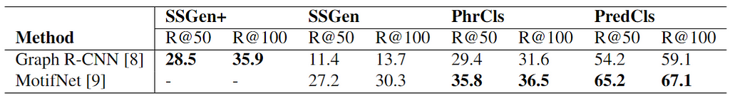
Quantitative Comparison: Both methods evaluated their model using the recall metric. Table 1 shows the comparison of both methods via different quantitative indicators. (1) Predicate Classification (PredCls) denotes the performance to recognize the relation between objects, (2) Phrase Classification (PhrCls) or scene graph classification in [9] depicts the ability to observe the categories of both objects and relations, (3) Scene Graph Generation (SGGen) or scene graph detection in [9] represents the performance to combine the objects with detected relations among them. In [8], they enhance the latter metric with a comprehensive SGGen (SGGen+) that includes the possibility of having a certain scenario like detecting a man as boy, technically it is a failed detection, but qualitatively if all the relations to this object is detected successfully then it should be considered as a successful result, hence increasing the SGGen metric value.
According to table 1, MotifNet [9] performs comparatively better when analyzing objects, edges, and relation labels separately. However, the generation of the entire graph of a given image is more accurate using the second approach, Graph R-CNN [8]. It also shows that having the comprehensive output metric shows a better analysis of the scene graph model.
Qualitative Comparison: In neural motifs structure [9], they consider the qualitative results separately. For instance, the detection of relation edge wearing as wears falls under the category of failed detection. It shows that the model [9] performs better than what the output metric number shows. On the other hand, [8] includes this understanding of result in their comprehensive SGGen (SGGen+) metric which already takes possible not-so-failed detections into consideration.
5. Applications in Robotics
This article will overview the understanding of scenes that helps in robotic applications, especially robot planning. The wide area of robotics including automatic indoor mapping, teleoperation robots, human-robot control for purposes like telemedicine, and many more results in a very deep area of SGs applications.
When both humans and robots collaborated in a similar workspace to complete a specified task, then it is called Human-Robot Collaboration (HRC), and the collaborative robots are called cobots. Having semantic information along with object detection makes the tasks even easier to do. [5] shows a method that uses SGG for safety analysis in HRC. Another application involves teleoperation robots that include social interaction skills like a meeting chat room on a mobile stick controlled by a human from a remote location. The applications include elderly care, attending events even if a person is disabled, etc. [2] discusses a method where scene understanding helps the user to analyze and control remote environment clearly.
5.1 Robot Planning
Assigning certain motion tasks to a robot, such as moving one object from one place to another, and expecting smooth service from a machine requires a highly accurate level of planning and development. SGG plays an important role in producing service robots as it gives the robot an in-depth abstracted picture of the scene which further helps it to locate objects precisely. [1] uses local scene graphs to perceive the global view to reach its target. It describes robot planning for a common task that includes searching for an object, such as a fruit, in an indoor environment.
Scene analysis for robot planning (SARP) [1] is an algorithm designed for robots to use visual contextual information to complete the planned task. This method takes advantage of scene graphs to model the global scene understanding using MotifNet [9], the algorithm discussed in section 3.2. The block diagram of the model can be accessed in [1]. The model uses MotifNet to generate local scene graphs, then the contextual information to analyze uncertainty between observations and actions, and update the robot’s belief. The latter process is done using the Partially Observable Markov Decision Process (PO-MDP) framework. The MDPs are known for sequential decision-making. In the block diagram, the offline trained scene graph network generates the global scene graphs and feeds the result into the Markov process.
Multiple Local SGs — — — — — →Global Context SGs — — — — →Target Search
The method is experimented for locating objects scattered through the area with precision and in minimal time. The robot is fed with a scene graph dataset, an already trained scene graph network, and a domain map for directive mobility. As a result, the robot navigates through the area for target search, and to do so, it creates scene graphs for contextual information every step of the way, as clearly shown in figure 2 and 3 of the published IEEE article [1]. It is the demonstration where the robot is assigned the task of locating a banana. It increments the global scene graph at every time instant except at T=4 because there are no new objects’ instances in that frame. It can be seen that having local scene graphs helped the robot to determine the global context for the target search. According to the performance comparison in [1], SARP outperforms the baseline methods both in terms of success rate and action cost. However, the model can be further expanded with facial recognition of humans, and also analyzed when changing or adding objects during the test process.
6. Conclusion
The article discusses the different methods for SGG, the generation of graphs having semantic information about scenes, and some of its robotic applications. The object and relation contextual information gives us a very descriptive understanding of a scene. MotifNet detects and adds the relation among objects as edge context using the LSTM network, while Graph R-CNN forms the scene graphs by eliminating the unlikely relation edges using relatedness score. There are several versions of the Visual Genome dataset used in recent approaches, however, MotifNet and Graph R-CNN evaluate their model on the same dataset model, which makes their quantitative comparison reasonable. Overall, both the quantitative and qualitative measurements are analyzed and it can be seen that numbers don’t tell the whole story, the not-so-failed scenarios, such as man instead of boy, should also be considered as successful outcome, if all of its relation edges are detected correctly, while evaluating a method for SGG. The applications in robotics is growing rapidly over the past decades and having an in-depth semantic description of the image, or scene will help in several image and video-related applications. One method is extensively discussed for the robot planning application that uses scene graphs for better visual scene understanding so that the robot can perform tasks (e.g., locating objects in indoor environment) in the long run.
Well, this is so much for a small research talk about converting images into interactive graphical texts. I hope you guys had fun (maybe a little!). I’ll be back with another research article summing up recent cool researches (probably on any topic from communication networking, Network Simulator (NS3), or maybe Wi-Fi 7😉).
Have fun researching!!
Regards,
Ritanshi
REFERENCES
- S. Amiri, K. Chandan, and S. Zhang. Reasoning with scene graphs for robot planning under partial observability. IEEE Robotics and Automation Letters, 7(2):5560–5567, 2022.
- F. Amodeo, F. Caballero, N. Díaz-Rodríguez, and L. Merino. Og-sgg: Ontology-guided scene graph generation. a case study in transfer learning for telepresence robotics. IEEE Access, pages 1–1, 2022.
- X. Chang, P. Ren, P. Xu, Z. Li, X. Chen, and A. Hauptmann. A comprehensive survey of scene graphs: Generation and application. IEEE Transactions on Pattern Analysis and Machine Intelligence, 45(1):1–26, 2023.
- R. Krishna, Y. Zhu, O. Groth, J. Johnson, K. Hata, J. Kravitz, S. Chen, Y. Kalantidis, L.-J. Li, D. A. Shamma, et al. Visual genome: Connecting language and vision using crowdsourced dense image annotations. International journal of computer vision, 123(1):32–73, 2017.
- H. Riaz, A. Terra, K. Raizer, R. Inam, and A. Hata. Scene understanding for safety analysis in human-robot collaborative operations. In 2020 6th International Conference on Control, Automation and Robotics (ICCAR), pages 722–731, 2020.
- M. Suhail, A. Mittal, B. Siddiquie, C. Broaddus, J. Eledath, G. Medioni, and L. Sigal. Energy-based learning for scene graph generation. In 2021 IEEE/CVF Conference on Computer Vision and Pattern Recognition (CVPR), pages 13931–13940, 2021.
- D. Xu, Y. Zhu, C. B. Choy, and L. Fei-Fei. Scene graph generation by iterative message passing. In Proceedings of the IEEE conference on computer vision and pattern recognition, pages 5410–5419, 2017.
- J. Yang, J. Lu, S. Lee, D. Batra, and D. Parikh. Graph r-cnn for scene graph generation. In Proceedings of the European conference on computer vision (ECCV), pages 670–685, 2018.
- R. Zellers, M. Yatskar, S. Thomson, and Y. Choi. Neural motifs: Scene graph parsing with global context. In 2018 IEEE/CVF Conference on Computer Vision and Pattern Recognition, pages 5831–5840, 2018.
- G. Zhu, L. Zhang, Y. Jiang, Y. Dang, H. Hou, P. Shen, M. Feng, X. Zhao, Q. Miao, S. A. A. Shah, et al. Scene graph generation: A comprehensive survey. arXiv preprint arXiv:2201.00443, 2022.
Scene Graph Generation and its Application in Robotics was originally published in Towards Data Science on Medium, where people are continuing the conversation by highlighting and responding to this story.
Let’s have a small talk about visualizing images with interactive graphical representation!
Scene graph generation is the process of generating scene graphs and a scene graph contains the visual understanding of an image in the form of a graph. It has nodes and edges representing the objects and their relationships, respectively. Contextual information about the scenes can help in semantic scene understanding. Although there are certain challenges such as uncertainty of real-world scenarios or unavailability of a standard dataset, researchers are trying to apply the scene graphs in the field of robotics. This write-up contains two major parts: one is about how scene graphs can be obtained by having an in-depth discussion about two state-of-the-art approaches for scene graph generation based on region-based convolutional neural networks, and the other part deals with the application of scene graphs in robot planning. In its former part, this article further explains that only having a numerical metric for model evaluation is insufficient for proper performance analysis. The latter part includes a thorough explanation of a method that uses the concept of scene graphs for visual context-aware robot planning.
1. Introduction
When considering the description of image elements in words, well-known active techniques such as image segmentation, object classification, activity identification, etc. play a significant role in the process. Scene Graph Generation (SGG) is a method to generate scene graphs (SGs), by depicting objects (e.g., humans, animals, etc.) and their attributes (e.g., color, clothes, vehicles, etc.) as nodes, and the relationships among objects as the edges. Fig. 1a and 1b shows how a scene graph generated from an RGB image usually looks like. It can be seen that the distinct colored nodes depict different major objects in the image (a male, a female, and a vehicle), the information about these objects is shown by the nodes having the variant of the same node color, and the edges are labeled with verbs showing a connection, or we can say relation among the nodes. The research has been going on for past years to make the SGs possible even for small details in the image.
This article extensively discusses two approaches in the upcoming sections for a better understanding of generating scene graphs. The write-up structure comprises six sections. The brief start of SGG and its prior applications including image and video captioning is explained in section 2. Section 3 describes the state-of-the-art methods with their model description. The experimental analysis of these methods is discussed and compared in section 4. Section 5 discusses some possible applications of SGs in the field of robotics with a main focus on robot planning, and also how having accurate SGs will make applications like telepresence robots, human-robot collaboration, etc. much easier to implement. Finally, section 6 concludes the entire literature.
2. Related Work
The SGs have a history of distinct applications, for instance, image and video captioning, visual question answering, 3D scene understanding, many applications in robotics, etc. [10] [3]. Most of the recent approaches include machine learning methods like Region-based Convolutional Neural Networks (R-CNN) [8], faster R-CNN [9], Recurrent Neural Networks (RNN) [7], etc. [7] proposed a structure that takes the image as input, then passes messages containing contextual information, and refines the prediction using RNN. Another method [6] uses the energy model of the image to generate comprehensive scene graphs. The datasets for SGG are also obtained using different real-world scenarios, images, and videos. The dataset mentioned here is a subset [7] of Visual Genome [4] containing 108,073 human-annotated images.
3. State-of-the-Art Approaches
3.1 Graph R-CNN Approach
J. Yang et. al. [8] proposes a model that first considers all the objects connected by an edge, relationship, then nullifies the unlikely relationship using a parameter called relatedness. For instance, it is more likely to have a relation between car and wheel, than a building and a wheel.
The paper shows a novel framework, namely Graph R-CNN with the introduction of a new evaluation metric, SGGen+. The model consists of three blocks, first to extract object nodes, second to remove unlikely edges, and finally to propagate graph context throughout the remaining graph so that the final scene graph can be produced. The novelty resides in the second and third block of the model, having a new relation proposal network (RePN) which computes relatedness that further helps in removing unlikely relationships, also called relation edge pruning and an attentional graph convolutional network (aGCN) that constitutes the propagation of higher-order context that leads to an update in scene graph giving it a final touch, respectively. Basically, the final block labeled the generated scene graph. The probability distribution of the whole idea can be depicted by the equation below, where for image I, O is the set of objects, R is the relation among objects, and Rl and Ol are relation and object labels respectively.
Pr(G|I) = Pr(O|I) * Pr(R|O, I) * Pr(Rl, Ol|O, R, I)
Fig. 2 shows the entire algorithm in pictorial form, and how all three stages work consecutively. The pipeline can be described as: using faster R-CNN for object detection, then generating an initial graph with all defined relationships, then pruning unlikely edges based on relatedness score, and then finally using aGCN for refining.
3.2 Stacked Motif Network (MotifNet)
R. Zellers et. al. [9] proposes a network that performs bounding box collection, object identification, and relation identification consecutively. The method shows the intense use of faster R-CNN and Long Short-term Memory (LSTM) networks. In contrast with Graph R-CNN, this method is based on detecting the relationships among objects and adding the relationship edges.
The idea here can be seen as a conditional probability equation, as shown in the equation below, which states the probability to find graph G of image I is given as the product of the probability of finding bounding box array B given I, probability of obtaining object O given B and I, and the probability of getting relations R among O given B, O and I.
Pr(G|I) = Pr(B|I) * Pr(O|B,I) * Pr(R|B,O,I)
Firstly, to find the set of the bounding box, they also use faster R-CNN, as in [8], shown on the left side of Fig. 3. It uses the VGG backbone structure for object identification while determining bounding boxes in I. Then, the model proceeds further with bidirectional LSTM layers depicted by the object context layer in Fig. 3. This block of layers generates the object labels for each bounding box region, bi ∈ B. Another bidirectional LSTM layers block is again used for determining relations as edge context, portrayed in the same figure. The output is computed as determining the edge labels which clearly depict the outer product with objects and relations among them. The detailed model structure can be learned in [9].
4. Experiments in State-of-the-Art Approaches
4.1 Experimental Setup
The setup for both methods is described below:
Graph R-CNN: The use of faster R-CNN with VGG16 backbone to ensure object detection is implemented via PyTorch. For the RePN implementation, a multi-layer perceptron structure is used to analyze the relatedness score using two projection functions, each for subject and object relation. Two aGCN layers are used, one for the feature level, the result of which is sent to the other one at the semantic level. The training is done in two stages, first only the object detector is trained, and then the whole model is trained jointly.
MotifNet: The images that are fed into the bounding box detector are made to be of size 592×592, by using the zero-padding method. All the LSTM layers undergo highway connections. Two and four alternating highway LSTM layers are used for object and edge context respectively. The ordering of the bounding box regions can be done in several ways using central x-coordinate, maximum non-background prediction, size of the bounding box, or just random shuffling.
The main challenge is to analyze the model with a common dataset framework, as different approaches use different data preprocessing, split, and evaluation. However, the discussed approaches, Graph R-CNN and MotifNet uses the publicly available data processing scheme and split from [7]. There are 150 object classes and 50 classes for relations in this Visual Genome dataset [4].
Visual Genome Dataset [4] in a nutshell:
Human Annotated Images
More than 100,000 images
150 Object Classes
50 Relation Classes
Each image has around 11.5 objects and 6.2 relationships in scene graph
4.2 Experimental Results
Quantitative Comparison: Both methods evaluated their model using the recall metric. Table 1 shows the comparison of both methods via different quantitative indicators. (1) Predicate Classification (PredCls) denotes the performance to recognize the relation between objects, (2) Phrase Classification (PhrCls) or scene graph classification in [9] depicts the ability to observe the categories of both objects and relations, (3) Scene Graph Generation (SGGen) or scene graph detection in [9] represents the performance to combine the objects with detected relations among them. In [8], they enhance the latter metric with a comprehensive SGGen (SGGen+) that includes the possibility of having a certain scenario like detecting a man as boy, technically it is a failed detection, but qualitatively if all the relations to this object is detected successfully then it should be considered as a successful result, hence increasing the SGGen metric value.
According to table 1, MotifNet [9] performs comparatively better when analyzing objects, edges, and relation labels separately. However, the generation of the entire graph of a given image is more accurate using the second approach, Graph R-CNN [8]. It also shows that having the comprehensive output metric shows a better analysis of the scene graph model.
Qualitative Comparison: In neural motifs structure [9], they consider the qualitative results separately. For instance, the detection of relation edge wearing as wears falls under the category of failed detection. It shows that the model [9] performs better than what the output metric number shows. On the other hand, [8] includes this understanding of result in their comprehensive SGGen (SGGen+) metric which already takes possible not-so-failed detections into consideration.
5. Applications in Robotics
This article will overview the understanding of scenes that helps in robotic applications, especially robot planning. The wide area of robotics including automatic indoor mapping, teleoperation robots, human-robot control for purposes like telemedicine, and many more results in a very deep area of SGs applications.
When both humans and robots collaborated in a similar workspace to complete a specified task, then it is called Human-Robot Collaboration (HRC), and the collaborative robots are called cobots. Having semantic information along with object detection makes the tasks even easier to do. [5] shows a method that uses SGG for safety analysis in HRC. Another application involves teleoperation robots that include social interaction skills like a meeting chat room on a mobile stick controlled by a human from a remote location. The applications include elderly care, attending events even if a person is disabled, etc. [2] discusses a method where scene understanding helps the user to analyze and control remote environment clearly.
5.1 Robot Planning
Assigning certain motion tasks to a robot, such as moving one object from one place to another, and expecting smooth service from a machine requires a highly accurate level of planning and development. SGG plays an important role in producing service robots as it gives the robot an in-depth abstracted picture of the scene which further helps it to locate objects precisely. [1] uses local scene graphs to perceive the global view to reach its target. It describes robot planning for a common task that includes searching for an object, such as a fruit, in an indoor environment.
Scene analysis for robot planning (SARP) [1] is an algorithm designed for robots to use visual contextual information to complete the planned task. This method takes advantage of scene graphs to model the global scene understanding using MotifNet [9], the algorithm discussed in section 3.2. The block diagram of the model can be accessed in [1]. The model uses MotifNet to generate local scene graphs, then the contextual information to analyze uncertainty between observations and actions, and update the robot’s belief. The latter process is done using the Partially Observable Markov Decision Process (PO-MDP) framework. The MDPs are known for sequential decision-making. In the block diagram, the offline trained scene graph network generates the global scene graphs and feeds the result into the Markov process.
Multiple Local SGs — — — — — →Global Context SGs — — — — →Target Search
The method is experimented for locating objects scattered through the area with precision and in minimal time. The robot is fed with a scene graph dataset, an already trained scene graph network, and a domain map for directive mobility. As a result, the robot navigates through the area for target search, and to do so, it creates scene graphs for contextual information every step of the way, as clearly shown in figure 2 and 3 of the published IEEE article [1]. It is the demonstration where the robot is assigned the task of locating a banana. It increments the global scene graph at every time instant except at T=4 because there are no new objects’ instances in that frame. It can be seen that having local scene graphs helped the robot to determine the global context for the target search. According to the performance comparison in [1], SARP outperforms the baseline methods both in terms of success rate and action cost. However, the model can be further expanded with facial recognition of humans, and also analyzed when changing or adding objects during the test process.
6. Conclusion
The article discusses the different methods for SGG, the generation of graphs having semantic information about scenes, and some of its robotic applications. The object and relation contextual information gives us a very descriptive understanding of a scene. MotifNet detects and adds the relation among objects as edge context using the LSTM network, while Graph R-CNN forms the scene graphs by eliminating the unlikely relation edges using relatedness score. There are several versions of the Visual Genome dataset used in recent approaches, however, MotifNet and Graph R-CNN evaluate their model on the same dataset model, which makes their quantitative comparison reasonable. Overall, both the quantitative and qualitative measurements are analyzed and it can be seen that numbers don’t tell the whole story, the not-so-failed scenarios, such as man instead of boy, should also be considered as successful outcome, if all of its relation edges are detected correctly, while evaluating a method for SGG. The applications in robotics is growing rapidly over the past decades and having an in-depth semantic description of the image, or scene will help in several image and video-related applications. One method is extensively discussed for the robot planning application that uses scene graphs for better visual scene understanding so that the robot can perform tasks (e.g., locating objects in indoor environment) in the long run.
Well, this is so much for a small research talk about converting images into interactive graphical texts. I hope you guys had fun (maybe a little!). I’ll be back with another research article summing up recent cool researches (probably on any topic from communication networking, Network Simulator (NS3), or maybe Wi-Fi 7😉).
Have fun researching!!
Regards,
Ritanshi
REFERENCES
- S. Amiri, K. Chandan, and S. Zhang. Reasoning with scene graphs for robot planning under partial observability. IEEE Robotics and Automation Letters, 7(2):5560–5567, 2022.
- F. Amodeo, F. Caballero, N. Díaz-Rodríguez, and L. Merino. Og-sgg: Ontology-guided scene graph generation. a case study in transfer learning for telepresence robotics. IEEE Access, pages 1–1, 2022.
- X. Chang, P. Ren, P. Xu, Z. Li, X. Chen, and A. Hauptmann. A comprehensive survey of scene graphs: Generation and application. IEEE Transactions on Pattern Analysis and Machine Intelligence, 45(1):1–26, 2023.
- R. Krishna, Y. Zhu, O. Groth, J. Johnson, K. Hata, J. Kravitz, S. Chen, Y. Kalantidis, L.-J. Li, D. A. Shamma, et al. Visual genome: Connecting language and vision using crowdsourced dense image annotations. International journal of computer vision, 123(1):32–73, 2017.
- H. Riaz, A. Terra, K. Raizer, R. Inam, and A. Hata. Scene understanding for safety analysis in human-robot collaborative operations. In 2020 6th International Conference on Control, Automation and Robotics (ICCAR), pages 722–731, 2020.
- M. Suhail, A. Mittal, B. Siddiquie, C. Broaddus, J. Eledath, G. Medioni, and L. Sigal. Energy-based learning for scene graph generation. In 2021 IEEE/CVF Conference on Computer Vision and Pattern Recognition (CVPR), pages 13931–13940, 2021.
- D. Xu, Y. Zhu, C. B. Choy, and L. Fei-Fei. Scene graph generation by iterative message passing. In Proceedings of the IEEE conference on computer vision and pattern recognition, pages 5410–5419, 2017.
- J. Yang, J. Lu, S. Lee, D. Batra, and D. Parikh. Graph r-cnn for scene graph generation. In Proceedings of the European conference on computer vision (ECCV), pages 670–685, 2018.
- R. Zellers, M. Yatskar, S. Thomson, and Y. Choi. Neural motifs: Scene graph parsing with global context. In 2018 IEEE/CVF Conference on Computer Vision and Pattern Recognition, pages 5831–5840, 2018.
- G. Zhu, L. Zhang, Y. Jiang, Y. Dang, H. Hou, P. Shen, M. Feng, X. Zhao, Q. Miao, S. A. A. Shah, et al. Scene graph generation: A comprehensive survey. arXiv preprint arXiv:2201.00443, 2022.
Scene Graph Generation and its Application in Robotics was originally published in Towards Data Science on Medium, where people are continuing the conversation by highlighting and responding to this story.
Denial of responsibility! Techno Blender is an automatic aggregator of the all world’s media. In each content, the hyperlink to the primary source is specified. All trademarks belong to their rightful owners, all materials to their authors. If you are the owner of the content and do not want us to publish your materials, please contact us by email – [email protected]. The content will be deleted within 24 hours.