Simulate a Tiny Solar System with Python | by Andrew Zhu | Jun, 2022

Simulate a tiny solar system with Sun, Earth, Mars, and an unknown comet using real mass, distance, and velocity data in Matplotlib

I was amazed by the PCA (Principal Components Analysis) and thinking of using animation to show the machine learning processes. When I managed to animate a graph, I was tempted to animate something cool. The first cool stuff that comes to me is the solar system. This article is also a journey of me recalling the knowledge of Newton’s physics, vector space, and matplotlib.

To simulate and animate the orbit of planets, I need to solve two key problems:

1. Generate the orbit data.
2. Animate the data with Matplotlib.

In this article, I am going to cover the above two problems. If you hurry and don’t want to read my long-winded gossip, you can check out the code host on Github.

All images and GIFs by the author.

According to Newton’s law of universal gravitation, we can calculate the force between two objects. Consider only earth and the sun. sun’s gravity force impact on earth can be represented by the equation:

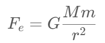
M denote the mass of the sun, m denote the mass of earth, r denote the distance between the center of two objects. G is a constant value.

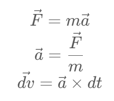
According to Newton’s second law:

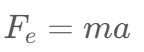
We can get the acceleration a:

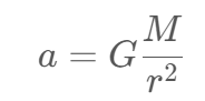
Hmm, the acceleration a is only related to the mass of the sun and the distance between the sun and earth r. Now with a known a. we can calculate the velocity of the earth after delta time – dt.

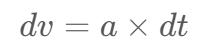
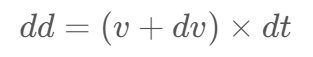
And finally, get the change of displacement — dd:

(I know it is annoying to use/read so many equations in an article, while this could be the easiest and most concise way to explain the foundation of gravitation orbit simulation)

Since I am going to plot the earth’s orbit with matplotlib, I need to calculate the value of x,y. For simplicity, I am going to use a 2D coordinate axis instead of 3D.

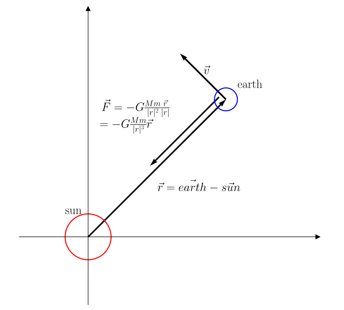
I drew the vector version of the equations in the above diagram. You may have several questions in mind if it is your first time reading the equation.

1. Why there is a minus (-) sign in the gravitation equation? Because the force direction is the opposite of the distance vector r. You will need to remove the minus sign (-) when you calculate the force put on the sun from the earth. In vector coordinate, we need to be very careful about directions.
2. What about centrifugal force, why don’t you deal with centrifugal force? Because the centrifugal force is actually the result of gravitation force. If we conduct force analysis on earth. there is only a gravitation force acting on it. When the earth is spinning around the sun, the earth is falling down to the sun. However, the earth’s initial velocity perpendicular to the G force pulls it away from the sun, that is why the earth can orbit the sun.

In Python code, assume the sun in position (0,0), earth in position (6,6):

sx,sy = 0,0
ex,ey = 6,6

The distance r will be:

rx = ex - sx
ry = ey - sy

Define GMm, the sun-earth gravity constant as gravconst_e:

Ms          = 2.0e30                    # mass of sun in kg unit
Me          = 5.972e24                  # mass of earth in kg unit        
G           = 6.67e-11
gravconst   = G*Ms*Me

The simulator will calculate a data point every dt time. we can set dt as one day:

daysec = 24.0*60*60
dt     = 1*daysec

The cube of r (|r|³) is:

modr3_e = (rx**2 + ry**2)**1.5

To calculate the force put on the earth’s direction:

# get g force in x and y direction
fx_e = gravconst_e*rx/modr3_e
fy_e = gravconst_e*ry/modr3_e

Based on Newton’s second law in vector form:

Combine the above equations:

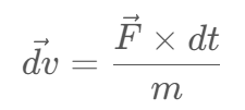
Since I have already calculated the force vector, I can get the new velocity vector after dt time:

xve += fx_e*dt/Me
yve += fy_e*dt/Me

Finally, get the earth’s new displacement (velocity multiply time is distance: d=v*t ):

xe += xve*dt
ye += yve*dt

Here is the full code that simulates the earth’s orbit for one year.

G           = 6.67e-11                  # constant G
Ms          = 2.0e30                    # sun
Me          = 5.972e24                  # earth        
AU          = 1.5e11                    # earth sun distance
daysec      = 24.0*60*60                # seconds of a day
e_ap_v      = 29290                     # earth velocity at apheliongravconst_e = G*Me*Ms
# setup the starting conditions
# earth
xe,ye,ze    = 1.0167*AU,0,0
xve,yve,zve = 0,e_ap_v,0# sun
xs,ys,zs    = 0,0,0
xvs,yvs,zvs = 0,0,0t           = 0.0
dt          = 1*daysec # every frame move this timexelist,yelist,zelist = [],[],[]
xslist,yslist,zslist = [],[],[]# start simulation
while t<1*365*daysec:
################ earth #############
# compute G force on earth
rx,ry,rz = xe - xs, ye - ys, ze - zs
modr3_e = (rx**2+ry**2+rz**2)**1.5
fx_e = -gravconst_e*rx/modr3_e
fy_e = -gravconst_e*ry/modr3_e
fz_e = -gravconst_e*rz/modr3_e
# update quantities how is this calculated?  F = ma -> a = F/m
xve += fx_e*dt/Me
yve += fy_e*dt/Me
zve += fz_e*dt/Me
# update position
xe += xve*dt
ye += yve*dt 
ze += zve*dt
# save the position in list
xelist.append(xe)
yelist.append(ye)
zelist.append(ze)
################ the sun ###########
# update quantities how is this calculated?  F = ma -> a = F/m
xvs += -fx_e*dt/Ms
yvs += -fy_e*dt/Ms
zvs += -fz_e*dt/Ms
# update position
xs += xvs*dt
ys += yvs*dt 
zs += zvs*dt
xslist.append(xs)
yslist.append(ys)
zslist.append(zs)
# update dt
t +=dt

To see what the orbit looks like:

import matplotlib.pyplot as plt
plt.plot(xelist,yelist,'-g',lw=2)
plt.axis('equal')
plt.show()

Now, I am going to turn the static earth track into a moving object with a trailing track preserved in the plane. Here are some of the problems I solved during building the animation:

1. All magic happens inside the update function. basically, the function will be called by FuncAnimation every frame. You can either call ax.plot(…)to draw new pixels in the plane (all pixels will be kept in the next frame) or call set_data or set_position to update the data of the visual object (matplotlib will redraw everything based on the data for the current frame).
2. The comma in the expression “line_e, = ax.plot(…)” looks weird in the beginning. But note that it is the comma that makes a tuple. “ax.plot(…)” returns a tuple object. That is why you will need to add a comma after the variable name.
3. To draw the tracking trailing after the earth. I initialize empty lists (exdata,eydata = [],[])to hold all previous track points. Append track point to the list every time when update function is called.

I am not going to turn this section into an animation tutorial. If you never tried matplotlib animation before. Jake VanderPlas’ Matplotlib Animation Tutorial is great to read.

Here is the code to animate the orbit:

import matplotlib.pyplot as plt
from matplotlib import animation
fig, ax = plt.subplots(figsize=(10,10))
ax.set_aspect('equal')
ax.grid()
line_e,     = ax.plot([],[],'-g',lw=1,c='blue')
point_e,    = ax.plot([AU], [0], marker="o"
, markersize=4
, markeredgecolor="blue"
, markerfacecolor="blue")
text_e      = ax.text(AU,0,'Earth')
point_s,    = ax.plot([0], [0], marker="o"
, markersize=7
, markeredgecolor="yellow"
, markerfacecolor="yellow")
text_s      = ax.text(0,0,'Sun')
exdata,eydata = [],[]                   # earth track
sxdata,sydata = [],[]                   # sun track
print(len(xelist))
def update(i):
exdata.append(xelist[i])
eydata.append(yelist[i])
line_e.set_data(exdata,eydata)
point_e.set_data(xelist[i],yelist[i])
text_e.set_position((xelist[i],yelist[i]))
point_s.set_data(xslist[i],yslist[i])
text_s.set_position((xslist[i],yslist[i]))
ax.axis('equal')
ax.set_xlim(-3*AU,3*AU)
ax.set_ylim(-3*AU,3*AU)
return line_e,point_s,point_e,text_e,text_s
anim = animation.FuncAnimation(fig
,func=update
,frames=len(xelist)
,interval=1
,blit=True)
plt.show()

Result:

Check out the full code here.

Change the initial earth velocity, say lower the earth’s velocity to 19,290 m/s (from 29,290 m/s):

Change the earth’s mass, increase it to 5.972e29 kg (from 5.972e24 kg). The sun is moving!

Since I have successfully simulated the earth’s and the sun’s orbit. it isn’t that hard to add more objects into the system. For example, Mars and an unknown comet.

Check out its code here.

With some tune on the plotting code, I can even animate the orbits in 3D! In the above simulation code, I already calculated the z axis data.

Check out the code here.

In this article, I went through the foundation of Newton’s gravitation law, how to convert the equations to vector space, and calculate the simulation data step by step. With simulation data in hand, I also explained three key problems on the way to animation.

Thank you for reading through here. With a thorough understanding of the simulation process, you can even build the famous Three-Body problem simulator. (yes, I am also a fan of the novel with the same name)

Let me know if you have any questions, I will try my best to answer them. And don’t hesitate to point out any mistakes I made in the article. looking forward to further connecting with you.

Let me stop here, wish you enjoy it and happy programming.

Before running the code, you will need to have LaTex installed on your machine.

import numpy as np
import matplotlib.pyplot as plt
plt.rcParams['text.usetex'] = True
font = {'family' : 'normal',
'weight' : 'bold',
'size'   : 18}
plt.rc('font',**font)
# initialize the stage
fig,ax = plt.subplots(figsize=(8,8))
# set x, and y axis,and remove top and right
ax.spines[['top','right']].set_visible(False)
ax.spines[['bottom','left']].set_position(('data',0.0))
ax.axis('equal')
ax.axes.xaxis.set_visible(False)
ax.axes.yaxis.set_visible(False)
ax.set_xlim(-3,10)
ax.set_ylim(-3,10)
# draw arrows
ax.plot(1, 0, ">k", transform=ax.get_yaxis_transform(), clip_on=False)
ax.plot(0, 1, "^k", transform=ax.get_xaxis_transform(), clip_on=False)
# sun
a = np.linspace(0,2*np.pi,360)
xs = np.sin(a)
ys = np.cos(a)
ax.plot(xs,ys,c='r')
ax.text(-1,1,'sun')
# earth
xec,yec = 6,6
xe = xec+ 0.5*xs
ye = yec+ 0.5*ys
ax.plot(xe,ye,c='b')
ax.text(xec+0.5,yec+0.5,'earth')
ax.text(xec-1,yec+1.1,r"$\vec{v}$")
# r vector
ax.quiver([0,xec,xec-0.3],[0,yec,yec+0.1]
,[xec,-2,-3],[yec,2,-3]
,units='xy',scale=1,width=0.07)
ax.text(3,2,r"$\vec{r} = \vec{earth}-\vec{sun}$")
f_eq = (r"$\vec{F}=-G\frac{Mm}{|r|^2}\frac{\vec{r}}{|r|}\\$"
r"$=-G\frac{Mm}{|r|^3}\vec{r}$")
ax.text(0.5,5.5,f_eq)
# plot data
plt.show()

Result:

Simulate a tiny solar system with Sun, Earth, Mars, and an unknown comet using real mass, distance, and velocity data in Matplotlib

I was amazed by the PCA (Principal Components Analysis) and thinking of using animation to show the machine learning processes. When I managed to animate a graph, I was tempted to animate something cool. The first cool stuff that comes to me is the solar system. This article is also a journey of me recalling the knowledge of Newton’s physics, vector space, and matplotlib.

To simulate and animate the orbit of planets, I need to solve two key problems:

1. Generate the orbit data.
2. Animate the data with Matplotlib.

In this article, I am going to cover the above two problems. If you hurry and don’t want to read my long-winded gossip, you can check out the code host on Github.

All images and GIFs by the author.

According to Newton’s law of universal gravitation, we can calculate the force between two objects. Consider only earth and the sun. sun’s gravity force impact on earth can be represented by the equation:

M denote the mass of the sun, m denote the mass of earth, r denote the distance between the center of two objects. G is a constant value.

According to Newton’s second law:

We can get the acceleration a:

Hmm, the acceleration a is only related to the mass of the sun and the distance between the sun and earth r. Now with a known a. we can calculate the velocity of the earth after delta time – dt.

And finally, get the change of displacement — dd:

(I know it is annoying to use/read so many equations in an article, while this could be the easiest and most concise way to explain the foundation of gravitation orbit simulation)

Since I am going to plot the earth’s orbit with matplotlib, I need to calculate the value of x,y. For simplicity, I am going to use a 2D coordinate axis instead of 3D.

I drew the vector version of the equations in the above diagram. You may have several questions in mind if it is your first time reading the equation.

1. Why there is a minus (-) sign in the gravitation equation? Because the force direction is the opposite of the distance vector r. You will need to remove the minus sign (-) when you calculate the force put on the sun from the earth. In vector coordinate, we need to be very careful about directions.
2. What about centrifugal force, why don’t you deal with centrifugal force? Because the centrifugal force is actually the result of gravitation force. If we conduct force analysis on earth. there is only a gravitation force acting on it. When the earth is spinning around the sun, the earth is falling down to the sun. However, the earth’s initial velocity perpendicular to the G force pulls it away from the sun, that is why the earth can orbit the sun.

In Python code, assume the sun in position (0,0), earth in position (6,6):

sx,sy = 0,0
ex,ey = 6,6

The distance r will be:

rx = ex - sx
ry = ey - sy

Define GMm, the sun-earth gravity constant as gravconst_e:

Ms          = 2.0e30                    # mass of sun in kg unit
Me          = 5.972e24                  # mass of earth in kg unit        
G           = 6.67e-11
gravconst   = G*Ms*Me

The simulator will calculate a data point every dt time. we can set dt as one day:

daysec = 24.0*60*60
dt     = 1*daysec

The cube of r (|r|³) is:

modr3_e = (rx**2 + ry**2)**1.5

To calculate the force put on the earth’s direction:

# get g force in x and y direction
fx_e = gravconst_e*rx/modr3_e
fy_e = gravconst_e*ry/modr3_e

Based on Newton’s second law in vector form:

Combine the above equations:

Since I have already calculated the force vector, I can get the new velocity vector after dt time:

xve += fx_e*dt/Me
yve += fy_e*dt/Me

Finally, get the earth’s new displacement (velocity multiply time is distance: d=v*t ):

xe += xve*dt
ye += yve*dt

Here is the full code that simulates the earth’s orbit for one year.

G           = 6.67e-11                  # constant G
Ms          = 2.0e30                    # sun
Me          = 5.972e24                  # earth        
AU          = 1.5e11                    # earth sun distance
daysec      = 24.0*60*60                # seconds of a day
e_ap_v      = 29290                     # earth velocity at apheliongravconst_e = G*Me*Ms
# setup the starting conditions
# earth
xe,ye,ze    = 1.0167*AU,0,0
xve,yve,zve = 0,e_ap_v,0# sun
xs,ys,zs    = 0,0,0
xvs,yvs,zvs = 0,0,0t           = 0.0
dt          = 1*daysec # every frame move this timexelist,yelist,zelist = [],[],[]
xslist,yslist,zslist = [],[],[]# start simulation
while t<1*365*daysec:
################ earth #############
# compute G force on earth
rx,ry,rz = xe - xs, ye - ys, ze - zs
modr3_e = (rx**2+ry**2+rz**2)**1.5
fx_e = -gravconst_e*rx/modr3_e
fy_e = -gravconst_e*ry/modr3_e
fz_e = -gravconst_e*rz/modr3_e
# update quantities how is this calculated?  F = ma -> a = F/m
xve += fx_e*dt/Me
yve += fy_e*dt/Me
zve += fz_e*dt/Me
# update position
xe += xve*dt
ye += yve*dt 
ze += zve*dt
# save the position in list
xelist.append(xe)
yelist.append(ye)
zelist.append(ze)
################ the sun ###########
# update quantities how is this calculated?  F = ma -> a = F/m
xvs += -fx_e*dt/Ms
yvs += -fy_e*dt/Ms
zvs += -fz_e*dt/Ms
# update position
xs += xvs*dt
ys += yvs*dt 
zs += zvs*dt
xslist.append(xs)
yslist.append(ys)
zslist.append(zs)
# update dt
t +=dt

To see what the orbit looks like:

import matplotlib.pyplot as plt
plt.plot(xelist,yelist,'-g',lw=2)
plt.axis('equal')
plt.show()

Now, I am going to turn the static earth track into a moving object with a trailing track preserved in the plane. Here are some of the problems I solved during building the animation:

1. All magic happens inside the update function. basically, the function will be called by FuncAnimation every frame. You can either call ax.plot(…)to draw new pixels in the plane (all pixels will be kept in the next frame) or call set_data or set_position to update the data of the visual object (matplotlib will redraw everything based on the data for the current frame).
2. The comma in the expression “line_e, = ax.plot(…)” looks weird in the beginning. But note that it is the comma that makes a tuple. “ax.plot(…)” returns a tuple object. That is why you will need to add a comma after the variable name.
3. To draw the tracking trailing after the earth. I initialize empty lists (exdata,eydata = [],[])to hold all previous track points. Append track point to the list every time when update function is called.

I am not going to turn this section into an animation tutorial. If you never tried matplotlib animation before. Jake VanderPlas’ Matplotlib Animation Tutorial is great to read.

Here is the code to animate the orbit:

import matplotlib.pyplot as plt
from matplotlib import animation
fig, ax = plt.subplots(figsize=(10,10))
ax.set_aspect('equal')
ax.grid()
line_e,     = ax.plot([],[],'-g',lw=1,c='blue')
point_e,    = ax.plot([AU], [0], marker="o"
, markersize=4
, markeredgecolor="blue"
, markerfacecolor="blue")
text_e      = ax.text(AU,0,'Earth')
point_s,    = ax.plot([0], [0], marker="o"
, markersize=7
, markeredgecolor="yellow"
, markerfacecolor="yellow")
text_s      = ax.text(0,0,'Sun')
exdata,eydata = [],[]                   # earth track
sxdata,sydata = [],[]                   # sun track
print(len(xelist))
def update(i):
exdata.append(xelist[i])
eydata.append(yelist[i])
line_e.set_data(exdata,eydata)
point_e.set_data(xelist[i],yelist[i])
text_e.set_position((xelist[i],yelist[i]))
point_s.set_data(xslist[i],yslist[i])
text_s.set_position((xslist[i],yslist[i]))
ax.axis('equal')
ax.set_xlim(-3*AU,3*AU)
ax.set_ylim(-3*AU,3*AU)
return line_e,point_s,point_e,text_e,text_s
anim = animation.FuncAnimation(fig
,func=update
,frames=len(xelist)
,interval=1
,blit=True)
plt.show()

Result:

Check out the full code here.

Change the initial earth velocity, say lower the earth’s velocity to 19,290 m/s (from 29,290 m/s):

Change the earth’s mass, increase it to 5.972e29 kg (from 5.972e24 kg). The sun is moving!

Since I have successfully simulated the earth’s and the sun’s orbit. it isn’t that hard to add more objects into the system. For example, Mars and an unknown comet.

Check out its code here.

With some tune on the plotting code, I can even animate the orbits in 3D! In the above simulation code, I already calculated the z axis data.

Check out the code here.

In this article, I went through the foundation of Newton’s gravitation law, how to convert the equations to vector space, and calculate the simulation data step by step. With simulation data in hand, I also explained three key problems on the way to animation.

Thank you for reading through here. With a thorough understanding of the simulation process, you can even build the famous Three-Body problem simulator. (yes, I am also a fan of the novel with the same name)

Let me know if you have any questions, I will try my best to answer them. And don’t hesitate to point out any mistakes I made in the article. looking forward to further connecting with you.

Let me stop here, wish you enjoy it and happy programming.

Before running the code, you will need to have LaTex installed on your machine.

import numpy as np
import matplotlib.pyplot as plt
plt.rcParams['text.usetex'] = True
font = {'family' : 'normal',
'weight' : 'bold',
'size'   : 18}
plt.rc('font',**font)
# initialize the stage
fig,ax = plt.subplots(figsize=(8,8))
# set x, and y axis,and remove top and right
ax.spines[['top','right']].set_visible(False)
ax.spines[['bottom','left']].set_position(('data',0.0))
ax.axis('equal')
ax.axes.xaxis.set_visible(False)
ax.axes.yaxis.set_visible(False)
ax.set_xlim(-3,10)
ax.set_ylim(-3,10)
# draw arrows
ax.plot(1, 0, ">k", transform=ax.get_yaxis_transform(), clip_on=False)
ax.plot(0, 1, "^k", transform=ax.get_xaxis_transform(), clip_on=False)
# sun
a = np.linspace(0,2*np.pi,360)
xs = np.sin(a)
ys = np.cos(a)
ax.plot(xs,ys,c='r')
ax.text(-1,1,'sun')
# earth
xec,yec = 6,6
xe = xec+ 0.5*xs
ye = yec+ 0.5*ys
ax.plot(xe,ye,c='b')
ax.text(xec+0.5,yec+0.5,'earth')
ax.text(xec-1,yec+1.1,r"$\vec{v}$")
# r vector
ax.quiver([0,xec,xec-0.3],[0,yec,yec+0.1]
,[xec,-2,-3],[yec,2,-3]
,units='xy',scale=1,width=0.07)
ax.text(3,2,r"$\vec{r} = \vec{earth}-\vec{sun}$")
f_eq = (r"$\vec{F}=-G\frac{Mm}{|r|^2}\frac{\vec{r}}{|r|}\\$"
r"$=-G\frac{Mm}{|r|^3}\vec{r}$")
ax.text(0.5,5.5,f_eq)
# plot data
plt.show()

Result: