
Smart Distributed Training on Amazon SageMaker with SMD: Part 2 | by Chaim Rand | Sep, 2022
How to Optimize Data Distribution with SageMaker Distributed Data Parallel
This is the second part of a three-part post on the topic of optimizing distributed training. In part one, we provided a brief survey of distributed training algorithms. We noted that common to all algorithms is their reliance on high-speed communication between multiple GPUs. We surmised that a distributed algorithm that accounted for the underlying instance topology, particularly the differences in the communication links between GPU pairs, would perform better than one that did not.
In part two we will demonstrate how to use Amazon SageMaker’s distributed data parallel (SDP) library to perform data distribution in a way that distinguishes between intra-node and inter-node GPU-to-GPU communication.
In data distributed training each GPU maintains its own copy of the model and alignment between the copies is preserved through gradient sharing. A good data distribution algorithm will implement the gradient sharing mechanism in a way that limits the impact on the training throughput. Some gradient sharing algorithms rely on one or more central parameter servers that collect gradient updates from all of the workers and then broadcast the results back to the workers. Others rely on direct peer-to-peer communication between the GPUs. A popular algorithm for gradient sharing is Ring-AllReduce in which multiple messages pass between workers in a one-directional ring. See here for a great visual review of how Ring-AllReduce works. Ring-AllReduce is used by Horovod, a popular framework for data distributed training.
The Amazon SageMaker distributed data parallel (SDP) library aims to simplify and accelerate data distributed training. You can see more details about SDP in the feature announcement, in the Amazon SageMaker Developer Guide, and in the associated white paper. (Anyone who wondered how the cover image I chose is relevant to the contents of this post need look no further than the title of the white paper: Herring: Rethinking the parameter server at scale for the cloud.) SDP’s gradient sharing algorithm relies on a number of crafty techniques. The property most relevant to our discussion in this post, is the distinction that is made between intra-node GPU-to-GPU communication and inter-node GPU-to-GPU communication. This distinction is summarized in the image below that shows a two-tier process in which intra-node GPUs share gradients via NVLink, whereas communication between GPUs of different nodes is mediated via servers on the CPUs of all of the nodes in use.
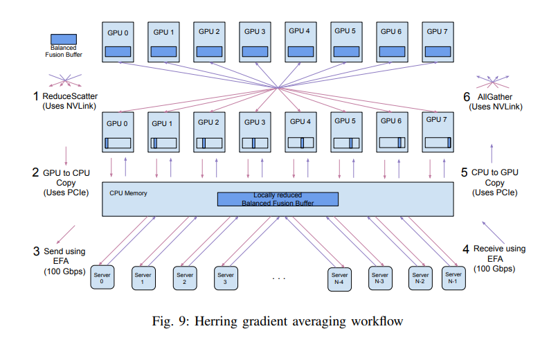
The white paper demonstrates how this kind of approach, that is a distributed algorithm that is tailored to the topology of the underlying training environment, can speed up high scale distributed training jobs when compared to the standard Ring-AllReduce algorithm.
We should note that in addition to the hierarchical gradient distribution algorithm used by SDP, there are several additional algorithms and libraries that offer solutions that account for the underlying instance topology. For example, despite having popularized the use of Ring-AllReduce, Horovod too supports a hierarchical gradient sharing algorithm. It also exposes controls for tuning the gradient flow based on the project and environment details. In addition, the underlying NCCL operations which are used by Horovod, also include advanced hierarchical techniques.
One advantage that SDP has over other libraries is with regards to instance topology discovery. The details of the training environment such as network bandwidths and latency are important inputs into choosing the best gradient sharing algorithm. Being that SDP is built into the SageMaker framework, it has immediate and detailed knowledge of the instance topology. Other libraries are not privy to the same level of detail and may be forced to either guess the best gradient sharing strategy or attempt to discover the missing information and tune accordingly.
Example
Here we show an example of integrating SDP into a simple TensorFlow (2.9) script. The SageMaker documentation includes a number of TensorFlow examples demonstrating the invocation of the SMP APIs. In our example we will include two helpful techniques currently absent from the SageMaker examples:
- How to program your scripts so that you can easily toggle between SDP and the popular Horovod library.
- How to combine SDP with the TensorFlow’s high level API for model training — tf.keras.Model.fit(). While the high level API hides access to the TensorFlow GradientTape, SDP requires that it be wrapped with tensorflow.DistributedGradientTape API. We overcome this conflict by customizing the training step of the model.fit() call.
The example is comprised of two scripts. The distributed training job start-up script and the training script.
The first script is the SageMaker training session start-up script. In this example we have chosen to set the input mode to Fast File Mode, an Amazon SageMaker feature that enables streaming input data directly from Amazon S3 to the training instances. The data is stored in TFRecord files. Although typically distributed training will run on particularly large datasets, for this example I created the files from the CIFAR-10 dataset (using this script). The session is instantiated with four p4d.24xlarge training instances and the distribution setting is configured to use the SageMaker data distribution library.
from sagemaker.tensorflow import TensorFlow
from sagemaker.session import TrainingInputs3_input = TrainingInput(
's3://'+S3_BUCKET_DATASET+'/cifar10-tfrecord/',
input_mode='FastFile')# Training using SMDataParallel Distributed Training Framework
distribution = {'smdistributed':
{'dataparallel':{'enabled': True}}
}tensorflow = TensorFlow(entry_point='train_tf.py',
role=<role>,
instance_type='ml.p4d.24xlarge',
instance_count=4,
framework_version='2.9.1',
py_version='py39',
distribution=distribution)tensorflow.fit(s3_input, job_name='data-parallel-example')
Note that the same script can be modified to start up a Horovod session by modifying only the distribution setting:
distribution = {
'mpi': {
'enabled': True,
'processes_per_host': 8
}
}
The second script includes the training loop. We have designed the script so as to demonstrate just how easy it is to convert between using the Horovod data distribution framework and the Amazon SageMaker data parallel library. The script begins with a run_hvd switch that can be used to toggle between the two options. The subsequent if-else block contains the only library specific code. As discussed above, we have implemented a custom training step that uses the DistributedGradientTape API.
import tensorflow as tf# toggle flag to run Horovod
run_hvd = False
if run_hvd:
import horovod.tensorflow as dist
from horovod.tensorflow.keras.callbacks import \
BroadcastGlobalVariablesCallback
else:
import smdistributed.dataparallel.tensorflow as dist
from tensorflow.keras.callbacks import Callback
class BroadcastGlobalVariablesCallback(Callback):
def __init__(self, root_rank, *args):
super(BroadcastGlobalVariablesCallback, self).
__init__(*args)
self.root_rank = root_rank
self.broadcast_done = False def on_batch_end(self, batch, logs=None):
if self.broadcast_done:
return
dist.broadcast_variables(self.model.variables,
root_rank=self.root_rank)
dist.broadcast_variables(self.model.optimizer.variables(),
root_rank=self.root_rank)
self.broadcast_done = True# Create Custom Model that performs the train step using
# DistributedGradientTapefrom keras.engine import data_adapter
class CustomModel(tf.keras.Model):
def train_step(self, data):
x, y, w = data_adapter.unpack_x_y_sample_weight(data)
with tf.GradientTape() as tape:
y_pred = self(x, training=True)
loss = self.compute_loss(x, y, y_pred, w)
tape = dist.DistributedGradientTape(tape)
self._validate_target_and_loss(y, loss)
self.optimizer.minimize(loss,
self.trainable_variables,
tape=tape)
return self.compute_metrics(x, y, y_pred, w)def get_dataset(batch_size, rank):
def parse_sample(example_proto):
image_feature_description = {
'image': tf.io.FixedLenFeature([], tf.string),
'label': tf.io.FixedLenFeature([], tf.int64)
}
features = tf.io.parse_single_example(example_proto,
image_feature_description)
image = tf.io.decode_raw(features['image'], tf.uint8)
image.set_shape([3 * 32 * 32])
image = tf.reshape(image, [32, 32, 3])
image = tf.cast(image, tf.float32)/255.
label = tf.cast(features['label'], tf.int32)
return image, label aut = tf.data.experimental.AUTOTUNE
records = tf.data.Dataset.list_files(
os.environ.get("SM_CHANNEL_TRAINING")+'/*',
shuffle=True)
ds = tf.data.TFRecordDataset(records, num_parallel_reads=aut)
ds = ds.repeat()
ds = ds.map(parse_sample, num_parallel_calls=aut)
ds = ds.batch(batch_size)
ds = ds.prefetch(aut)
return dsif __name__ == "__main__":
import argparse, os
parser = argparse.ArgumentParser(description="Train resnet")
parser.add_argument("--model_dir", type=str,
default="./model_keras_resnet")
args = parser.parse_args()# init distribution lib
outputs = tf.keras.applications.ResNet50(weights=None,
dist.init()
gpus = tf.config.experimental.list_physical_devices('GPU')
for gpu in gpus:
tf.config.experimental.set_memory_growth(gpu, True)
if gpus:
tf.config.experimental.set_visible_devices(
gpus[dist.local_rank()], 'GPU')
input_shape = (32, 32, 3)
classes = 10
inputs = tf.keras.Input(shape=input_shape)
input_shape=input_shape,
classes=classes)(inputs)
model = CustomModel(inputs, outputs)
model.compile(loss=tf.losses.SparseCategoricalCrossentropy(),
optimizer= tf.optimizers.Adam())
dataset = get_dataset(batch_size = 1024, rank=dist.local_rank())
cbs = [BroadcastGlobalVariablesCallback(0)]
model.fit(dataset, steps_per_epoch=100,
epochs=10, callbacks=cbs, verbose=2)
Results
In this section we compare the runtime results of performing distributed training with the Horovod data distribution framework and the Amazon SageMaker data parallel library. The runtime performance was measured by the average number of seconds per training step.
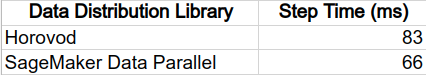
Our experiment shows that the environment-aware distributed training algorithms of the SDP library outperform the algorithms used by the Horovod library by roughly 20%. Note that the comparative performance will vary greatly based on the details of your project and based on the instance configuration you choose. Even for the same project and same instance configuration, results may differ based on the precise placement of the instances in your training job. As noted above, instances can be placed in different cluster placement groups which may increase latency and slow training.
Please note that as of the time of this writing, SDP is not supported on all instance types. See the documentation for details.
In the third and final part of our post we will demonstrate how Amazon SageMaker’s distributed data parallel library supports data distribution in a way that distinguishes between intra-node and inter-node GPU pairs.
How to Optimize Data Distribution with SageMaker Distributed Data Parallel
This is the second part of a three-part post on the topic of optimizing distributed training. In part one, we provided a brief survey of distributed training algorithms. We noted that common to all algorithms is their reliance on high-speed communication between multiple GPUs. We surmised that a distributed algorithm that accounted for the underlying instance topology, particularly the differences in the communication links between GPU pairs, would perform better than one that did not.
In part two we will demonstrate how to use Amazon SageMaker’s distributed data parallel (SDP) library to perform data distribution in a way that distinguishes between intra-node and inter-node GPU-to-GPU communication.
In data distributed training each GPU maintains its own copy of the model and alignment between the copies is preserved through gradient sharing. A good data distribution algorithm will implement the gradient sharing mechanism in a way that limits the impact on the training throughput. Some gradient sharing algorithms rely on one or more central parameter servers that collect gradient updates from all of the workers and then broadcast the results back to the workers. Others rely on direct peer-to-peer communication between the GPUs. A popular algorithm for gradient sharing is Ring-AllReduce in which multiple messages pass between workers in a one-directional ring. See here for a great visual review of how Ring-AllReduce works. Ring-AllReduce is used by Horovod, a popular framework for data distributed training.
The Amazon SageMaker distributed data parallel (SDP) library aims to simplify and accelerate data distributed training. You can see more details about SDP in the feature announcement, in the Amazon SageMaker Developer Guide, and in the associated white paper. (Anyone who wondered how the cover image I chose is relevant to the contents of this post need look no further than the title of the white paper: Herring: Rethinking the parameter server at scale for the cloud.) SDP’s gradient sharing algorithm relies on a number of crafty techniques. The property most relevant to our discussion in this post, is the distinction that is made between intra-node GPU-to-GPU communication and inter-node GPU-to-GPU communication. This distinction is summarized in the image below that shows a two-tier process in which intra-node GPUs share gradients via NVLink, whereas communication between GPUs of different nodes is mediated via servers on the CPUs of all of the nodes in use.
The white paper demonstrates how this kind of approach, that is a distributed algorithm that is tailored to the topology of the underlying training environment, can speed up high scale distributed training jobs when compared to the standard Ring-AllReduce algorithm.
We should note that in addition to the hierarchical gradient distribution algorithm used by SDP, there are several additional algorithms and libraries that offer solutions that account for the underlying instance topology. For example, despite having popularized the use of Ring-AllReduce, Horovod too supports a hierarchical gradient sharing algorithm. It also exposes controls for tuning the gradient flow based on the project and environment details. In addition, the underlying NCCL operations which are used by Horovod, also include advanced hierarchical techniques.
One advantage that SDP has over other libraries is with regards to instance topology discovery. The details of the training environment such as network bandwidths and latency are important inputs into choosing the best gradient sharing algorithm. Being that SDP is built into the SageMaker framework, it has immediate and detailed knowledge of the instance topology. Other libraries are not privy to the same level of detail and may be forced to either guess the best gradient sharing strategy or attempt to discover the missing information and tune accordingly.
Example
Here we show an example of integrating SDP into a simple TensorFlow (2.9) script. The SageMaker documentation includes a number of TensorFlow examples demonstrating the invocation of the SMP APIs. In our example we will include two helpful techniques currently absent from the SageMaker examples:
- How to program your scripts so that you can easily toggle between SDP and the popular Horovod library.
- How to combine SDP with the TensorFlow’s high level API for model training — tf.keras.Model.fit(). While the high level API hides access to the TensorFlow GradientTape, SDP requires that it be wrapped with tensorflow.DistributedGradientTape API. We overcome this conflict by customizing the training step of the model.fit() call.
The example is comprised of two scripts. The distributed training job start-up script and the training script.
The first script is the SageMaker training session start-up script. In this example we have chosen to set the input mode to Fast File Mode, an Amazon SageMaker feature that enables streaming input data directly from Amazon S3 to the training instances. The data is stored in TFRecord files. Although typically distributed training will run on particularly large datasets, for this example I created the files from the CIFAR-10 dataset (using this script). The session is instantiated with four p4d.24xlarge training instances and the distribution setting is configured to use the SageMaker data distribution library.
from sagemaker.tensorflow import TensorFlow
from sagemaker.session import TrainingInputs3_input = TrainingInput(
's3://'+S3_BUCKET_DATASET+'/cifar10-tfrecord/',
input_mode='FastFile')# Training using SMDataParallel Distributed Training Framework
distribution = {'smdistributed':
{'dataparallel':{'enabled': True}}
}tensorflow = TensorFlow(entry_point='train_tf.py',
role=<role>,
instance_type='ml.p4d.24xlarge',
instance_count=4,
framework_version='2.9.1',
py_version='py39',
distribution=distribution)tensorflow.fit(s3_input, job_name='data-parallel-example')
Note that the same script can be modified to start up a Horovod session by modifying only the distribution setting:
distribution = {
'mpi': {
'enabled': True,
'processes_per_host': 8
}
}
The second script includes the training loop. We have designed the script so as to demonstrate just how easy it is to convert between using the Horovod data distribution framework and the Amazon SageMaker data parallel library. The script begins with a run_hvd switch that can be used to toggle between the two options. The subsequent if-else block contains the only library specific code. As discussed above, we have implemented a custom training step that uses the DistributedGradientTape API.
import tensorflow as tf# toggle flag to run Horovod
run_hvd = False
if run_hvd:
import horovod.tensorflow as dist
from horovod.tensorflow.keras.callbacks import \
BroadcastGlobalVariablesCallback
else:
import smdistributed.dataparallel.tensorflow as dist
from tensorflow.keras.callbacks import Callback
class BroadcastGlobalVariablesCallback(Callback):
def __init__(self, root_rank, *args):
super(BroadcastGlobalVariablesCallback, self).
__init__(*args)
self.root_rank = root_rank
self.broadcast_done = False def on_batch_end(self, batch, logs=None):
if self.broadcast_done:
return
dist.broadcast_variables(self.model.variables,
root_rank=self.root_rank)
dist.broadcast_variables(self.model.optimizer.variables(),
root_rank=self.root_rank)
self.broadcast_done = True# Create Custom Model that performs the train step using
# DistributedGradientTapefrom keras.engine import data_adapter
class CustomModel(tf.keras.Model):
def train_step(self, data):
x, y, w = data_adapter.unpack_x_y_sample_weight(data)
with tf.GradientTape() as tape:
y_pred = self(x, training=True)
loss = self.compute_loss(x, y, y_pred, w)
tape = dist.DistributedGradientTape(tape)
self._validate_target_and_loss(y, loss)
self.optimizer.minimize(loss,
self.trainable_variables,
tape=tape)
return self.compute_metrics(x, y, y_pred, w)def get_dataset(batch_size, rank):
def parse_sample(example_proto):
image_feature_description = {
'image': tf.io.FixedLenFeature([], tf.string),
'label': tf.io.FixedLenFeature([], tf.int64)
}
features = tf.io.parse_single_example(example_proto,
image_feature_description)
image = tf.io.decode_raw(features['image'], tf.uint8)
image.set_shape([3 * 32 * 32])
image = tf.reshape(image, [32, 32, 3])
image = tf.cast(image, tf.float32)/255.
label = tf.cast(features['label'], tf.int32)
return image, label aut = tf.data.experimental.AUTOTUNE
records = tf.data.Dataset.list_files(
os.environ.get("SM_CHANNEL_TRAINING")+'/*',
shuffle=True)
ds = tf.data.TFRecordDataset(records, num_parallel_reads=aut)
ds = ds.repeat()
ds = ds.map(parse_sample, num_parallel_calls=aut)
ds = ds.batch(batch_size)
ds = ds.prefetch(aut)
return dsif __name__ == "__main__":
import argparse, os
parser = argparse.ArgumentParser(description="Train resnet")
parser.add_argument("--model_dir", type=str,
default="./model_keras_resnet")
args = parser.parse_args()# init distribution lib
outputs = tf.keras.applications.ResNet50(weights=None,
dist.init()
gpus = tf.config.experimental.list_physical_devices('GPU')
for gpu in gpus:
tf.config.experimental.set_memory_growth(gpu, True)
if gpus:
tf.config.experimental.set_visible_devices(
gpus[dist.local_rank()], 'GPU')
input_shape = (32, 32, 3)
classes = 10
inputs = tf.keras.Input(shape=input_shape)
input_shape=input_shape,
classes=classes)(inputs)
model = CustomModel(inputs, outputs)
model.compile(loss=tf.losses.SparseCategoricalCrossentropy(),
optimizer= tf.optimizers.Adam())
dataset = get_dataset(batch_size = 1024, rank=dist.local_rank())
cbs = [BroadcastGlobalVariablesCallback(0)]
model.fit(dataset, steps_per_epoch=100,
epochs=10, callbacks=cbs, verbose=2)
Results
In this section we compare the runtime results of performing distributed training with the Horovod data distribution framework and the Amazon SageMaker data parallel library. The runtime performance was measured by the average number of seconds per training step.
Our experiment shows that the environment-aware distributed training algorithms of the SDP library outperform the algorithms used by the Horovod library by roughly 20%. Note that the comparative performance will vary greatly based on the details of your project and based on the instance configuration you choose. Even for the same project and same instance configuration, results may differ based on the precise placement of the instances in your training job. As noted above, instances can be placed in different cluster placement groups which may increase latency and slow training.
Please note that as of the time of this writing, SDP is not supported on all instance types. See the documentation for details.
In the third and final part of our post we will demonstrate how Amazon SageMaker’s distributed data parallel library supports data distribution in a way that distinguishes between intra-node and inter-node GPU pairs.
Denial of responsibility! Techno Blender is an automatic aggregator of the all world’s media. In each content, the hyperlink to the primary source is specified. All trademarks belong to their rightful owners, all materials to their authors. If you are the owner of the content and do not want us to publish your materials, please contact us by email – [email protected]. The content will be deleted within 24 hours.