
Solving Differential Equations With Neural Networks
How Neural Networks are strong tools for solving differential equations without the use of training data
Differential equations are one of the protagonists in physical sciences, with vast applications in engineering, biology, economy, and even social sciences. Roughly speaking, they tell us how a quantity varies in time (or some other parameter, but usually we are interested in time variations). We can understand how a population, or a stock price, or even how the opinion of some society towards certain themes changes over time.
Typically, the methods used to solve DEs are not analytical (i.e. there is no "closed formula" for the solution) and we have to resource to numerical methods. However, numerical methods can be expensive from a computational standpoint, and worse than that: the accumulated error can be significantly large.
This article will showcase how a Neural Network can be a valuable ally to solve a differential equation, and how we can borrow concepts from Physics-Informed Neural Networks to tackle the question: can we use a machine learning approach to solve a DE?
A pinch of Physics-Informed Neural Networks
In this section, I will talk about Physics-Informed Neural Networks very briefly. I suppose you know the "neural network" part, but what makes them be informed by physics? Well, they are not exactly informed by physics, but rather by a (differential) equation.
Usually, neural networks are trained to find patterns and figure out what's going on with a set of training data. However, when you train a neural network to obey the behavior of your training data and hopefully fit unseen data, your model is highly dependent on the data itself, and not on the underlying nature of your system. It sounds almost like a philosophical matter, but it is more practical than that: if your data comes from measurements of ocean currents, these currents have to obey the physics equations that describe ocean currents. Notice, however, that your neural network is completely agnostic about these equations and is only trying to fit data points.
This is where physics informed comes into play. If, besides learning how to fit your data, your model also learns how to fit the equations that govern that system, the predictions of your neural network will be much more precise and will generalize much better, just citing some advantages of physics-informed models.
Notice that the governing equations of your system don't have to involve physics at all, the "physics-informed" thing is just nomenclature (and the technique is most used by physicists anyway). If your system is the traffic in a city and you happen to have a good mathematical model that you want your neural network's predictions to obey, then physics-informed neural networks are a good fit for you.
How do we inform these models?
Hopefully, I've convinced you that it is worth the trouble to make the model aware of the underlying equations that govern our system. However, how can we do this? There are several approaches to this, but the main one is to adapt the loss function to have a term that accounts for the governing equations, aside from the usual data-related part. That is, the loss function L will be composed of the sum

Here, the data loss is the usual one: a mean squared difference, or some other suited form of loss function; but the equation part is the charming one. Imagine that your system is governed by the following differential equation:

How can we fit this into the loss function? Well, since our task when training a neural network is to minimize the loss function, what we want is to minimize the following expression:

So our equation-related loss function turns out to be

that is, it is the mean difference squared of our DE. If we manage to minimize this (a.k.a. make this term as close to zero as possible) we automatically satisfy the system's governing equation. Pretty clever, right?
Now, the extra term L_IC in the loss function needs to be addressed: it accounts for the initial conditions of the system. If a system's initial conditions are not provided, there are infinitely many solutions for a differential equation. For instance, a ball thrown from the ground level has its trajectory governed by the same differential equation as a ball thrown from the 10th floor; however, we know for sure that the paths made by these balls will not be the same. What changes here are the initial conditions of the system. How does our model know which initial conditions we are talking about? It is natural at this point that we enforce it using a loss function term! For our DE, let's impose that when t = 0, y = 1. Hence, we want to minimize an initial condition loss function that reads:

If we minimize this term, then we automatically satisfy the initial conditions of our system. Now, what is left to be understood is how to use this to solve a differential equation.
Solving a differential equation
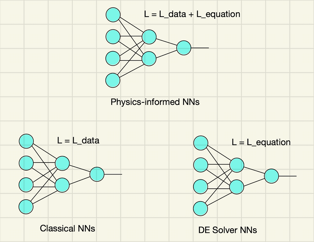
If a neural network can be trained either with the data-related term of the loss function (this is what is usually done in classical architectures), and can also be trained with both the data and the equation-related term (this is physics-informed neural networks I just mentioned), it must be true that it can be trained to minimize only the equation-related term. This is exactly what we are going to do! The only loss function used here will be the L_equation. Hopefully, this diagram below illustrates what I've just said: today we are aiming for the right-bottom type of model, our DE solver NN.
Code implementation
To showcase the theoretical learnings we've just got, I will implement the proposed solution in Python code, using the PyTorch library for machine learning.
The first thing to do is to create a neural network architecture:
import torch
import torch.nn as nn

class NeuralNet(nn.Module):
    def __init__(self, hidden_size, output_size=1,input_size=1):
        super(NeuralNet, self).__init__()
        self.l1 = nn.Linear(input_size, hidden_size)
        self.relu1 = nn.LeakyReLU()
        self.l2 = nn.Linear(hidden_size, hidden_size)
        self.relu2 = nn.LeakyReLU()
        self.l3 = nn.Linear(hidden_size, hidden_size)
        self.relu3 = nn.LeakyReLU()
        self.l4 = nn.Linear(hidden_size, output_size)

    def forward(self, x):
        out = self.l1(x)
        out = self.relu1(out)
        out = self.l2(out)
        out = self.relu2(out)
        out = self.l3(out)
        out = self.relu3(out)
        out = self.l4(out)
        return out
This one is just a simple MLP with LeakyReLU activation functions. Then, I will define the loss functions to calculate them later during the training loop:
# Create the criterion that will be used for the DE part of the loss
criterion = nn.MSELoss()

# Define the loss function for the initial condition
def initial_condition_loss(y, target_value):
    return nn.MSELoss()(y, target_value)
Now, we shall create a time array that will be used as train data, and instantiate the model, and also choose an optimization algorithm:
# Time vector that will be used as input of our NN
t_numpy = np.arange(0, 5+0.01, 0.01, dtype=np.float32)
t = torch.from_numpy(t_numpy).reshape(len(t_numpy), 1)
t.requires_grad_(True)

# Constant for the model
k = 1

# Instantiate one model with 50 neurons on the hidden layers
model = NeuralNet(hidden_size=50)

# Loss and optimizer
learning_rate = 8e-3
optimizer = torch.optim.SGD(model.parameters(), lr=learning_rate)

# Number of epochs
num_epochs = int(1e4)
Finally, let's start our training loop:
for epoch in range(num_epochs):

    # Randomly perturbing the training points to have a wider range of times
    epsilon = torch.normal(0,0.1, size=(len(t),1)).float()
    t_train = t + epsilon

    # Forward pass
    y_pred = model(t_train)

    # Calculate the derivative of the forward pass w.r.t. the input (t)
    dy_dt = torch.autograd.grad(y_pred,
                                t_train,
                                grad_outputs=torch.ones_like(y_pred),
                                create_graph=True)[0]

    # Define the differential equation and calculate the loss
    loss_DE = criterion(dy_dt + k*y_pred, torch.zeros_like(dy_dt))

    # Define the initial condition loss
    loss_IC = initial_condition_loss(model(torch.tensor([[0.0]])),
                                     torch.tensor([[1.0]]))

    loss = loss_DE + loss_IC

    # Backward pass and weight update
    optimizer.zero_grad()
    loss.backward()
    optimizer.step()
Notice the use of torch.autograd.grad function to automatically differentiate the output y_pred with respect to the input t to compute the loss function.
Results
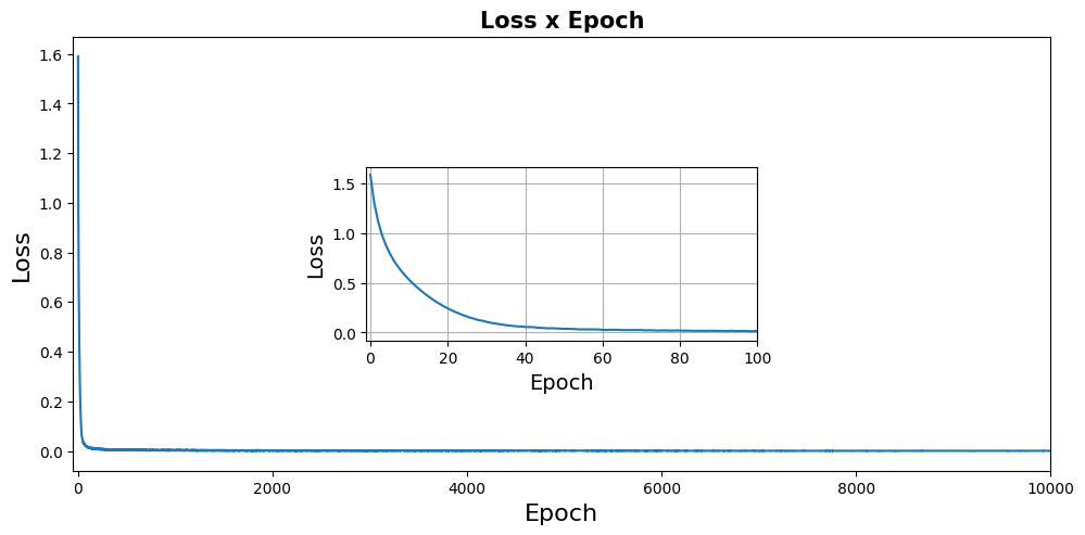
After training, we can see that the loss function rapidly converges. Fig. 2 shows the loss function plotted against the epoch number, with an inset showing the region where the loss function has its fastest drop.
You probably have noticed that this neural network is not a common one. It has no train data (our train data was a hand-crafted vector of timestamps, which is simply the time domain that we wanted to investigate), so all information it gets from the system comes in the form of a loss function. Its only purpose is to solve a differential equation within the time domain it was crafted to solve. Hence, to test it, it's only fair that we use the time domain it was trained on. Fig. 3 shows a comparison between the NN prediction and the theoretical answer (that is, the analytical solution).
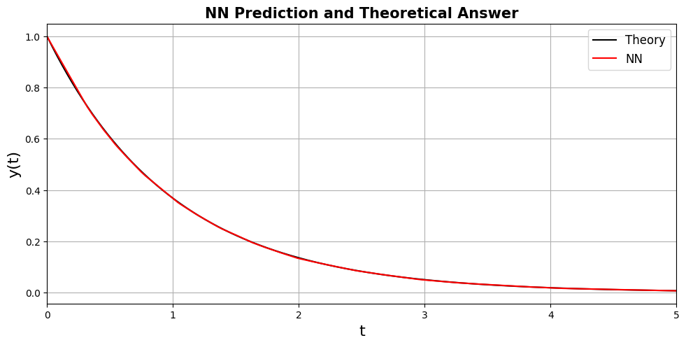
We can see a pretty good agreement between the two, which is very good for the neural network.
One caveat of this approach is that it does not generalize well for future times. Fig. 4 shows what happens if we slide our time data points five steps ahead, and the result is simply mayhem.
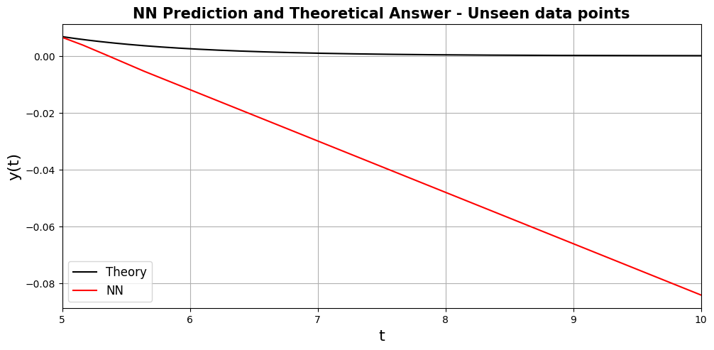
Hence, the lesson here is that this approach is made to be a numerical solver for differential equations within a time domain, and it should not be used as a regular neural network to make predictions with unseen out-of-train-domain data and expect it to generalize well.
Conclusion
After all, one remaining question is:
Why bother to train a neural network that does not generalize well to unseen data, and on top of that is obviously worse than the analytical solution, since it has an intrinsic statistical error?
First, the example provided here was an example of a differential equation whose analytical solution is known. For unknown solutions, numerical methods must be used nevertheless. With that being said, numerical methods for differential equation solving usually accumulate error. That means if you try to solve the equation for many time steps, the solution will lose its accuracy along the way. The neural network solver, on the other hand, learns how to solve the DE for all data points at each of its training epochs.
Another reason is that neural networks are good interpolators, so if you want to know the value of the function in unseen data (but this "unseen data" has to lie within the time interval you trained) the neural network will promptly give you a value that classic numeric methods will not be able to promptly give.
References
[1] Marios Mattheakis et al., Hamiltonian neural networks for solving equations of motion, arXiv preprint arXiv:2001.11107v5, 2022.
[2] Mario Dagrada, Introduction to Physics-informed Neural Networks, 2022.
Solving Differential Equations With Neural Networks was originally published in Towards Data Science on Medium, where people are continuing the conversation by highlighting and responding to this story.
How Neural Networks are strong tools for solving differential equations without the use of training data

Differential equations are one of the protagonists in physical sciences, with vast applications in engineering, biology, economy, and even social sciences. Roughly speaking, they tell us how a quantity varies in time (or some other parameter, but usually we are interested in time variations). We can understand how a population, or a stock price, or even how the opinion of some society towards certain themes changes over time.
Typically, the methods used to solve DEs are not analytical (i.e. there is no "closed formula" for the solution) and we have to resource to numerical methods. However, numerical methods can be expensive from a computational standpoint, and worse than that: the accumulated error can be significantly large.
This article will showcase how a Neural Network can be a valuable ally to solve a differential equation, and how we can borrow concepts from Physics-Informed Neural Networks to tackle the question: can we use a machine learning approach to solve a DE?
A pinch of Physics-Informed Neural Networks
In this section, I will talk about Physics-Informed Neural Networks very briefly. I suppose you know the "neural network" part, but what makes them be informed by physics? Well, they are not exactly informed by physics, but rather by a (differential) equation.
Usually, neural networks are trained to find patterns and figure out what's going on with a set of training data. However, when you train a neural network to obey the behavior of your training data and hopefully fit unseen data, your model is highly dependent on the data itself, and not on the underlying nature of your system. It sounds almost like a philosophical matter, but it is more practical than that: if your data comes from measurements of ocean currents, these currents have to obey the physics equations that describe ocean currents. Notice, however, that your neural network is completely agnostic about these equations and is only trying to fit data points.
This is where physics informed comes into play. If, besides learning how to fit your data, your model also learns how to fit the equations that govern that system, the predictions of your neural network will be much more precise and will generalize much better, just citing some advantages of physics-informed models.
Notice that the governing equations of your system don't have to involve physics at all, the "physics-informed" thing is just nomenclature (and the technique is most used by physicists anyway). If your system is the traffic in a city and you happen to have a good mathematical model that you want your neural network's predictions to obey, then physics-informed neural networks are a good fit for you.
How do we inform these models?
Hopefully, I've convinced you that it is worth the trouble to make the model aware of the underlying equations that govern our system. However, how can we do this? There are several approaches to this, but the main one is to adapt the loss function to have a term that accounts for the governing equations, aside from the usual data-related part. That is, the loss function L will be composed of the sum
Here, the data loss is the usual one: a mean squared difference, or some other suited form of loss function; but the equation part is the charming one. Imagine that your system is governed by the following differential equation:
How can we fit this into the loss function? Well, since our task when training a neural network is to minimize the loss function, what we want is to minimize the following expression:
So our equation-related loss function turns out to be
that is, it is the mean difference squared of our DE. If we manage to minimize this (a.k.a. make this term as close to zero as possible) we automatically satisfy the system's governing equation. Pretty clever, right?
Now, the extra term L_IC in the loss function needs to be addressed: it accounts for the initial conditions of the system. If a system's initial conditions are not provided, there are infinitely many solutions for a differential equation. For instance, a ball thrown from the ground level has its trajectory governed by the same differential equation as a ball thrown from the 10th floor; however, we know for sure that the paths made by these balls will not be the same. What changes here are the initial conditions of the system. How does our model know which initial conditions we are talking about? It is natural at this point that we enforce it using a loss function term! For our DE, let's impose that when t = 0, y = 1. Hence, we want to minimize an initial condition loss function that reads:
If we minimize this term, then we automatically satisfy the initial conditions of our system. Now, what is left to be understood is how to use this to solve a differential equation.
Solving a differential equation
If a neural network can be trained either with the data-related term of the loss function (this is what is usually done in classical architectures), and can also be trained with both the data and the equation-related term (this is physics-informed neural networks I just mentioned), it must be true that it can be trained to minimize only the equation-related term. This is exactly what we are going to do! The only loss function used here will be the L_equation. Hopefully, this diagram below illustrates what I've just said: today we are aiming for the right-bottom type of model, our DE solver NN.
Code implementation
To showcase the theoretical learnings we've just got, I will implement the proposed solution in Python code, using the PyTorch library for machine learning.
The first thing to do is to create a neural network architecture:
import torch
import torch.nn as nn

class NeuralNet(nn.Module):
    def __init__(self, hidden_size, output_size=1,input_size=1):
        super(NeuralNet, self).__init__()
        self.l1 = nn.Linear(input_size, hidden_size)
        self.relu1 = nn.LeakyReLU()
        self.l2 = nn.Linear(hidden_size, hidden_size)
        self.relu2 = nn.LeakyReLU()
        self.l3 = nn.Linear(hidden_size, hidden_size)
        self.relu3 = nn.LeakyReLU()
        self.l4 = nn.Linear(hidden_size, output_size)

    def forward(self, x):
        out = self.l1(x)
        out = self.relu1(out)
        out = self.l2(out)
        out = self.relu2(out)
        out = self.l3(out)
        out = self.relu3(out)
        out = self.l4(out)
        return out
This one is just a simple MLP with LeakyReLU activation functions. Then, I will define the loss functions to calculate them later during the training loop:
# Create the criterion that will be used for the DE part of the loss
criterion = nn.MSELoss()

# Define the loss function for the initial condition
def initial_condition_loss(y, target_value):
    return nn.MSELoss()(y, target_value)
Now, we shall create a time array that will be used as train data, and instantiate the model, and also choose an optimization algorithm:
# Time vector that will be used as input of our NN
t_numpy = np.arange(0, 5+0.01, 0.01, dtype=np.float32)
t = torch.from_numpy(t_numpy).reshape(len(t_numpy), 1)
t.requires_grad_(True)

# Constant for the model
k = 1

# Instantiate one model with 50 neurons on the hidden layers
model = NeuralNet(hidden_size=50)

# Loss and optimizer
learning_rate = 8e-3
optimizer = torch.optim.SGD(model.parameters(), lr=learning_rate)

# Number of epochs
num_epochs = int(1e4)
Finally, let's start our training loop:
for epoch in range(num_epochs):

    # Randomly perturbing the training points to have a wider range of times
    epsilon = torch.normal(0,0.1, size=(len(t),1)).float()
    t_train = t + epsilon

    # Forward pass
    y_pred = model(t_train)

    # Calculate the derivative of the forward pass w.r.t. the input (t)
    dy_dt = torch.autograd.grad(y_pred,
                                t_train,
                                grad_outputs=torch.ones_like(y_pred),
                                create_graph=True)[0]

    # Define the differential equation and calculate the loss
    loss_DE = criterion(dy_dt + k*y_pred, torch.zeros_like(dy_dt))

    # Define the initial condition loss
    loss_IC = initial_condition_loss(model(torch.tensor([[0.0]])),
                                     torch.tensor([[1.0]]))

    loss = loss_DE + loss_IC

    # Backward pass and weight update
    optimizer.zero_grad()
    loss.backward()
    optimizer.step()
Notice the use of torch.autograd.grad function to automatically differentiate the output y_pred with respect to the input t to compute the loss function.
Results
After training, we can see that the loss function rapidly converges. Fig. 2 shows the loss function plotted against the epoch number, with an inset showing the region where the loss function has its fastest drop.
You probably have noticed that this neural network is not a common one. It has no train data (our train data was a hand-crafted vector of timestamps, which is simply the time domain that we wanted to investigate), so all information it gets from the system comes in the form of a loss function. Its only purpose is to solve a differential equation within the time domain it was crafted to solve. Hence, to test it, it's only fair that we use the time domain it was trained on. Fig. 3 shows a comparison between the NN prediction and the theoretical answer (that is, the analytical solution).
We can see a pretty good agreement between the two, which is very good for the neural network.
One caveat of this approach is that it does not generalize well for future times. Fig. 4 shows what happens if we slide our time data points five steps ahead, and the result is simply mayhem.
Hence, the lesson here is that this approach is made to be a numerical solver for differential equations within a time domain, and it should not be used as a regular neural network to make predictions with unseen out-of-train-domain data and expect it to generalize well.
Conclusion
After all, one remaining question is:
Why bother to train a neural network that does not generalize well to unseen data, and on top of that is obviously worse than the analytical solution, since it has an intrinsic statistical error?
First, the example provided here was an example of a differential equation whose analytical solution is known. For unknown solutions, numerical methods must be used nevertheless. With that being said, numerical methods for differential equation solving usually accumulate error. That means if you try to solve the equation for many time steps, the solution will lose its accuracy along the way. The neural network solver, on the other hand, learns how to solve the DE for all data points at each of its training epochs.
Another reason is that neural networks are good interpolators, so if you want to know the value of the function in unseen data (but this "unseen data" has to lie within the time interval you trained) the neural network will promptly give you a value that classic numeric methods will not be able to promptly give.
References
[1] Marios Mattheakis et al., Hamiltonian neural networks for solving equations of motion, arXiv preprint arXiv:2001.11107v5, 2022.
[2] Mario Dagrada, Introduction to Physics-informed Neural Networks, 2022.
Solving Differential Equations With Neural Networks was originally published in Towards Data Science on Medium, where people are continuing the conversation by highlighting and responding to this story.
Denial of responsibility! Techno Blender is an automatic aggregator of the all world’s media. In each content, the hyperlink to the primary source is specified. All trademarks belong to their rightful owners, all materials to their authors. If you are the owner of the content and do not want us to publish your materials, please contact us by email – [email protected]. The content will be deleted within 24 hours.