
Solving the Travelling Salesman Problem for Germany using NetworkX in Python | by Himalaya Bir Shrestha | Jun, 2022
Discovering the shortest route to travel across the capital cities of 16 federal states of Germany while visiting each city once using the Christofides algorithm.
I have been residing in Germany for six years now. Germany is composed of 16 federal states, and I have visited five state capitals until now. Recently, a thought struck my mind:
I want to travel across the capital cities of all 16 federal states and visit each city exactly once while starting in Berlin and ending in Berlin. What would be the shortest possible route to do so?
This type of problem is known as a Travelling Salesman Problem (TSP). As the name suggests, a travelling salesman would go door to door, or region to region within a specified territory trying to sell the products or services of her/his business. The TSP deals with finding the shortest route covering all points exactly once since this would be the most effective route in terms of cost, time, and energy.
A decision problem is a problem having a “Yes” or “No” answer. There could be different complexity classes to solve it. Such as:
- P is a complexity class where the decision problem can be solved in polynomial time by a Deterministic Turing Machine (DTM). A polynomial-time algorithm has an execution time of the order O(nᵏ) for some nonnegative integer k, where n is the complexity of the input.
Problems that can be solved by a polynomial-time algorithm are called tractable problems. Examples of such algorithms are linear search (O(n)), binary search (O(log n)), insertion sort (O(n²)), merge sort (O(n log n)), and matrix multiplication (O(n³)) (Bari, 2018 and Maru, 2020).
- NP (Non-deterministic Polynomial-time) refers to a set of decision problems that can be solved in polynomial-time by a Non-deterministic Turing Machine (NTM). An NTM can have a group of actions to come to the solution, but the transition would be non-deterministic (randomised) for each execution (Tutorialspoint, 2022). Once a potential solution is provided for an NP problem, a DTM can verify its correctness in polynomial time (Viswarupan, 2016).
An algorithm, which is non-deterministic today can also be deterministic if someone finds its solution tomorrow (Bari, 2018 and Maru, 2020). This implies that a problem that can be solved by DTM in polynomial time can also be solved by NTM in polynomial time. Hence, P is a subset of NP.
- NP-hard is the complexity class of decision problems that are “at least as hard as the hardest problem in NP”. A problem H is NP-hard when every problem L in NP can be reduced in polynomial time to H; i.e., assuming a solution for H takes 1 unit time, H’s solution can be used to solve L in polynomial time. The solution of H and L (Yes or No) must also be the same.
TSP is an NP-hard problem. This implies that if there are a large number of cities, it is not feasible to evaluate every possible solution within a “reasonable” time (Hayes, 2019).
To solve the Travelling Salesman Problem (TSP), one needs to first understand the concept of the Hamilton cycle (also referred to as the Hamiltonian cycle). A Hamilton cycle is a graph cycle (closed loop) through a graph that visits each node exactly once (Mathworld, 2022a). This is named after Sir William Rowan Hamilton, who introduced this concept through a game called Hamiltonian puzzle (also known as the Icosian game).
In a graph with n nodes, the total number of possible Hamilton cycles is given by (n-1)! if we consider clockwise and anti-clockwise paths as two different paths. If we consider clockwise and anti-clockwise paths as the same, there are (n-1)!/2 possible Hamilton cycles.
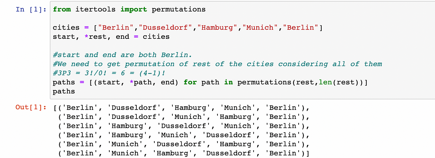
Let’s take an example of four cities: Berlin, Dusseldorf, Hamburg, and Munich. I aim to travel across these four cities starting and ending in Berlin while passing through the cities in between exactly once. The number of possible unique paths (Hamilton cycles) in this example is given by (4–1)! = 3! = 6.
In the code below, cities is a list of these four cities but with start and end as Berlin. The other three cities are defined as *rest. The permutation of these three cities taking all three at a time results in the all possible Hamilton cycles. This is shown in the Python code below.
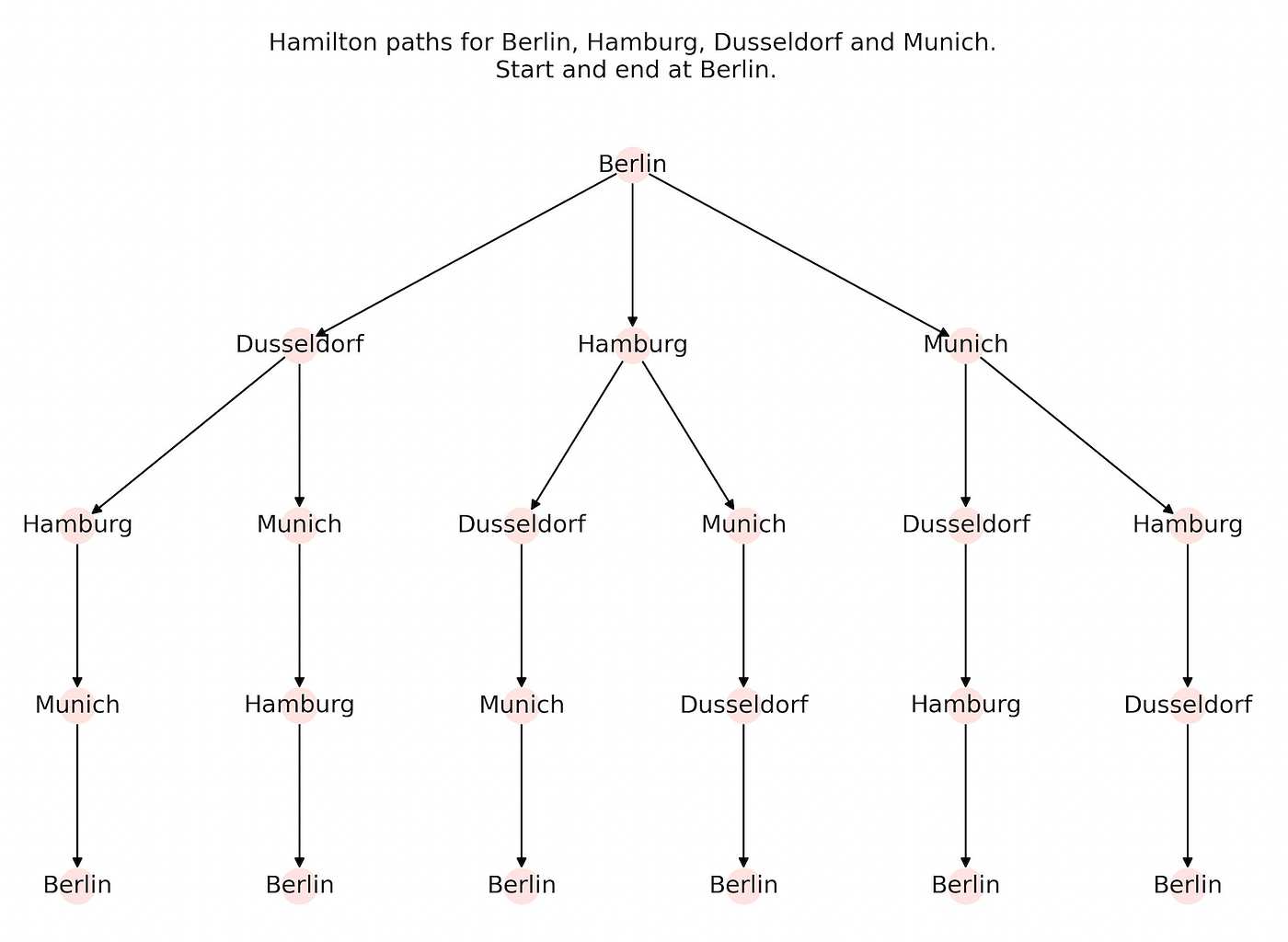
In the gist below, the make_tsp_tree function first creates a list of Hamilton paths, then creates a directed prefix tree from a list of those paths, and then returns the graph object G by removing the root node and the nil node. The position of each node in G is set using the dot layout of Graphviz, which sets hierarchical structure in directed graphs.
The Hamilton paths for the list of these four cities are presented in the graph below:
I define the list of 16 state capitals of Germany as capitals. Using a process called geocoding, I could get the coordinates of all 16 cities. The process of geocoding using the geopy package is described in detail in this story.
capitals = [‘Berlin’, ‘Bremen’, ‘Dresden’, ‘Dusseldorf’,
‘Erfurt’, ‘Hamburg’, ‘Hannover’, ‘Kiel’,
‘Magdeburg’, ‘Mainz’, ‘Munich’, ‘Potsdam’,   ‘Saarbrucken’, ‘Schwerin’, ‘Stuttgart’, ‘Wiesbaden’]
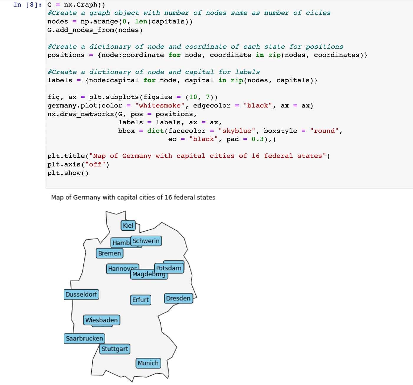
Using the GeoPandas package, I extract the map of Germany in GeoDataFrame called germany. To plot the capitals in germany, first I create a graph object G using NetworkX. Then I create 16 nodes, one for each city. Next, I create a dictionary of nodes and coordinates of each city for positions. And I create another dictionary of nodes and names of capital cities for labels. The code and the resulting map are given in the screenshot below.
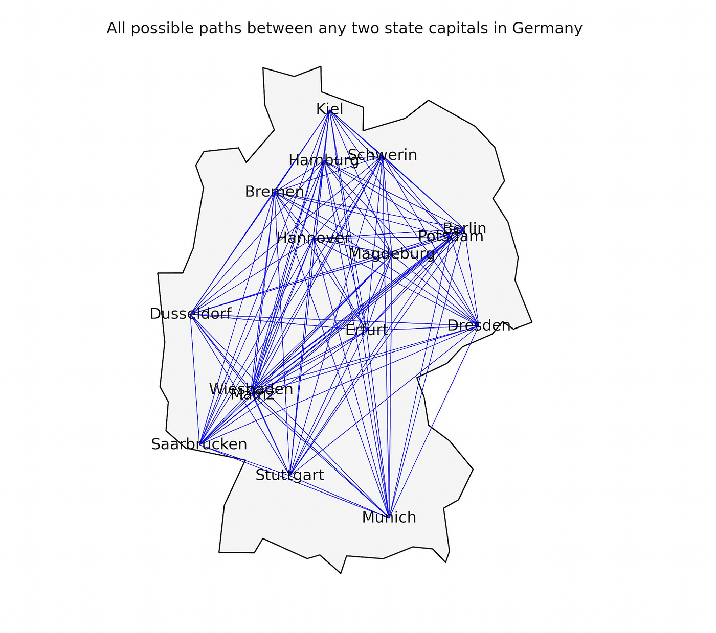
The next step is to determine and plot all the possible paths between any two cities in Germany. Since there are 16 cities in our list, the number of possible paths between any two cities is given by ⁿCᵣ = ¹⁶C₂ = 120. In the existing graph object G, I add the edges between any two nodes except itself as follows:
for i in nodes:
for j in nodes:
if i!=j:
G.add_edge(i, j)
Plotting the updated graph object G with germany with the recently added edges looks as follows:
I create H as a backup copy of G for later use.
Next, I calculate the Euclidean distance between all two cities in Germany, and this information is stored as the weights of the edges in G. Thus, G is now a complete weighted graph in which an edge connects each pair of graph nodes and each edge has a weight associated with it.
H = G.copy()#Calculating the distances between the nodes as edge's weight.
for i in range(len(pos)):
for j in range(i + 1, len(pos)):
#Multidimensional Euclidean distan
dist = math.hypot(pos[i][0] - pos[j][0], pos[i][1] - pos[j][1])
dist = dist
G.add_edge(i, j, weight=dist)
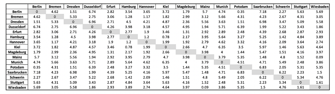
The distance between the cities with each other can be observed in the following table in the matrix format. In the following table, the distance between cities with themselves is zero as observed in the main diagonal. And all the entries above the main diagonal are reflected in the equal entries below the diagonal. Hence, it is an example of a hollow (zero-diagonal) symmetric matrix.
To find the solution cycle, NetworkX uses a default algorithm known as the Christofides algorithm for undirected graphs, and the list of edges that are part of the solution cycle is stored as edge_list. This is implemented in the code below:
cycle = nx_app.christofides(G, weight="weight")
edge_list = list(nx.utils.pairwise(cycle))
Christofides algorithm
The Christofides algorithm finds an approximate solution to the TSP, on instances where the distances form a metric space (they are symmetric and obey the triangle inequality, i.e., in ∆ABC, a+b≥c ) (Goodrich and Tamassia, 2014). This algorithm is named after a Cypriot mathematician named Nicos Christofides, who devised it in 1976. As of now, this algorithm offers the best approximation ratio to solve TSP (Christofides, 2022).
The basic steps of this algorithm are given below. These steps have been implemented in the source code of NetworkX here. I also illustrate the stepwise implementation of the algorithm for our problem.
- Find a minimum (weigh) spanning tree T of G.
The minimum spanning tree for a weighted, connected, undirected graph (here G) is a graph consisting of the subset of edges that together connect all connected nodes (here 16) while minimising the total sum of weights on the edges.
NetworkX uses a Kruskal algorithm to find the minimum spanning tree (NetworkX, 2015). This will look as follows in the case of Germany with the capital cities of its 16 federal states:

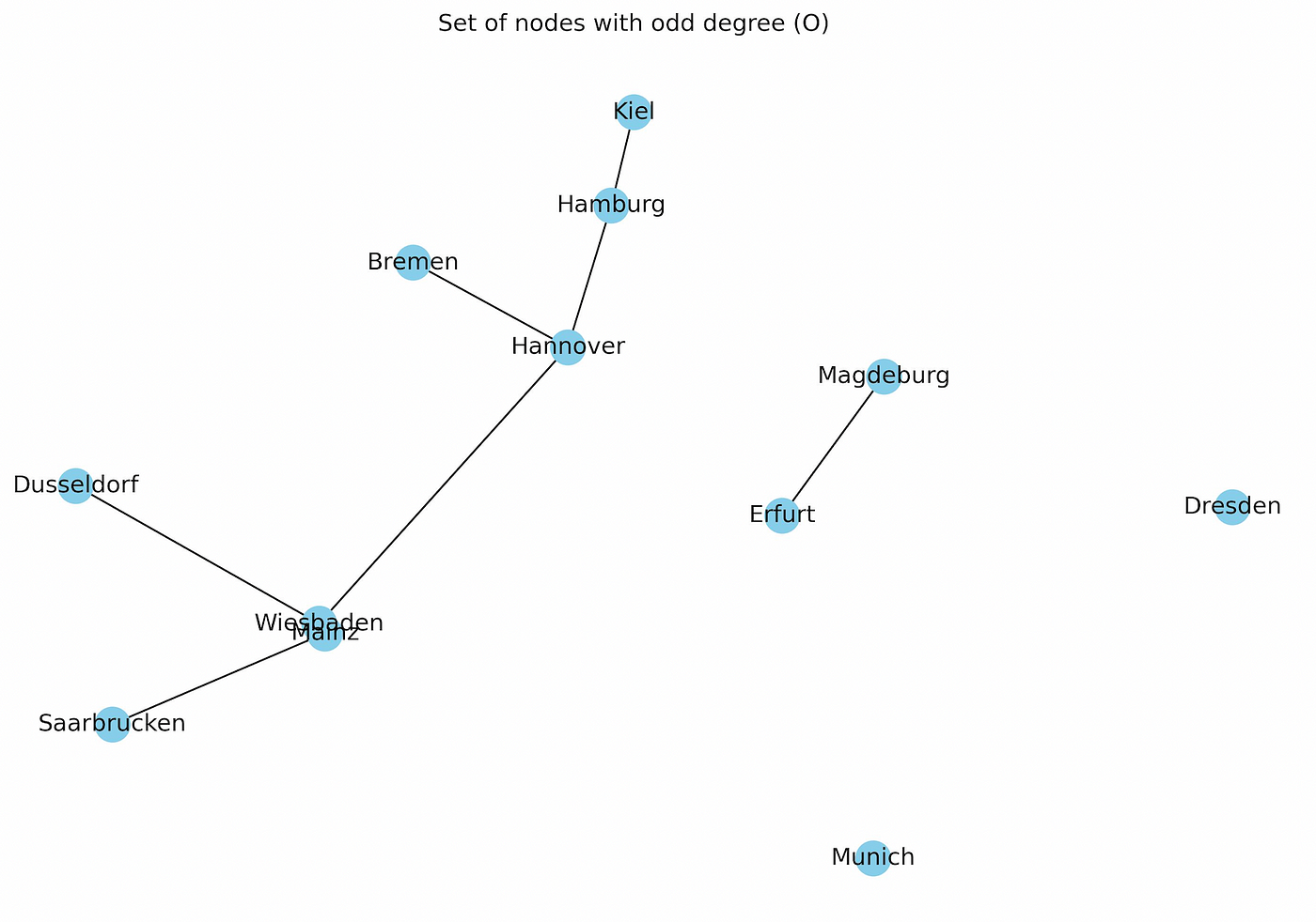
2. Make a set of nodes in T with an odd degree O.
In the next step, a set of nodes called O is created in which the degree of each node is odd. From the tree T above, we see that Berlin, Potsdam, Stuttgart, and Schwerin each have degree 2 i.e., even. Therefore, these nodes are removed in the new set O as shown below:
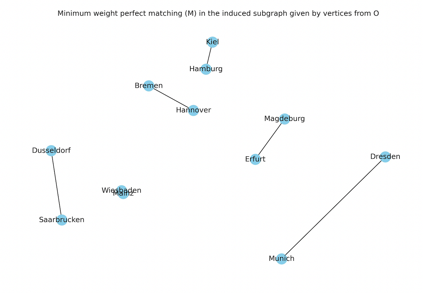
3. Find a minimum-weight perfect matching M in the induced subgraph given by the vertices from O.
To have a perfect matching, there needs to be an even number of nodes in a graph and each node is connected with exactly one other node. A perfect matching is therefore a matching containing n/2 edges (the largest possible) (Mathworld, 2022b).
The minimum weight perfect matching M computes a perfect matching which minimises the weight of matched edges as shown in the plot below.
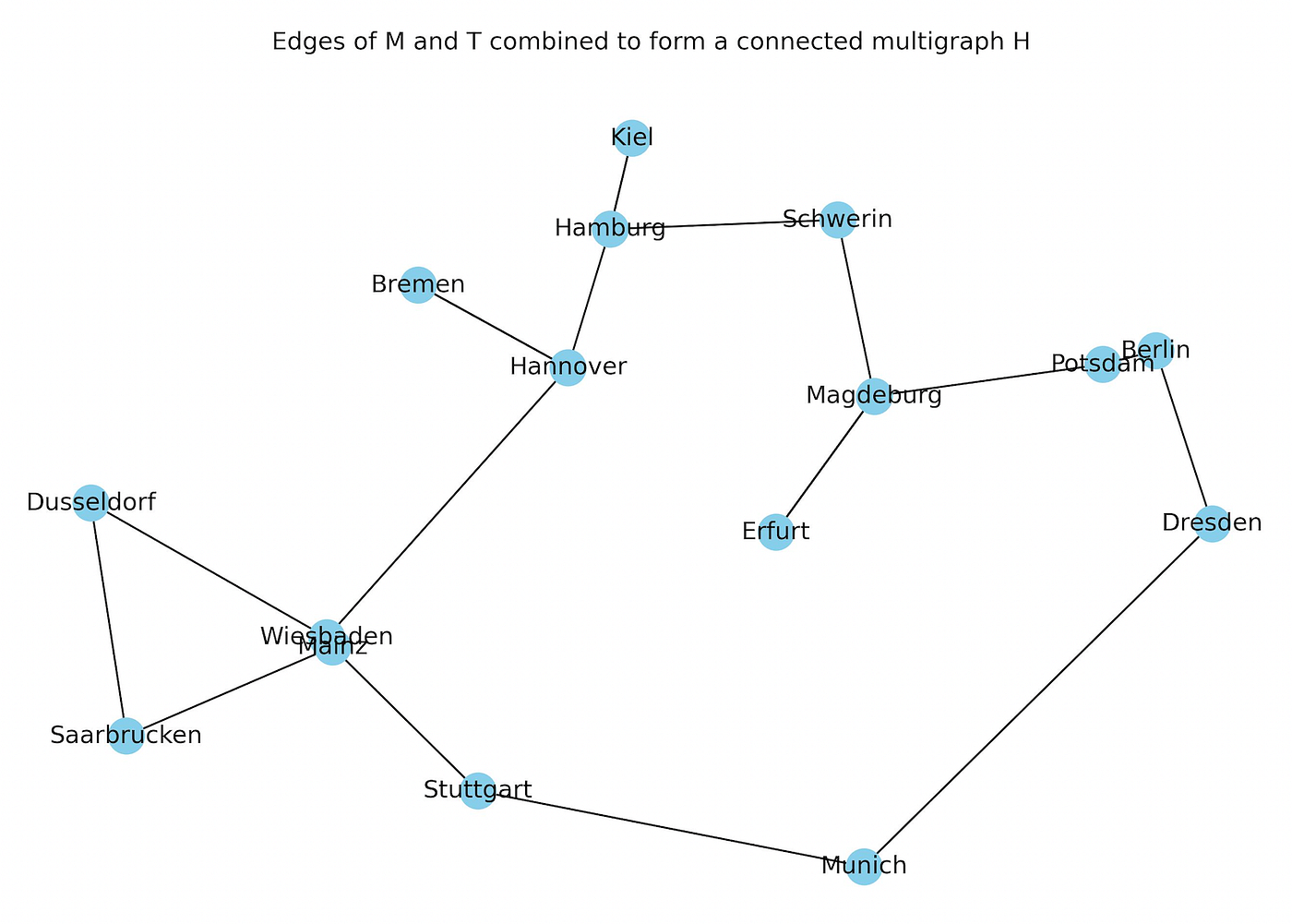
4. Combine the edges of M and T to form a connected multigraph H.
In the next step, the algorithm combines the edges of T in step 1 with M in step 3 to form a connected multigraph H.
5. Build an Eulerian circuit using the edges of M and T.
In the next step, the Christofides algorithm builds an Eulerian circuit using the edges of M and T. An Eulerian circuit is a trail in a finite graph that visits each edge exactly once. Each node in an Eulerian circuit must have an even degree (MIT OpenCourseWare, 2016). The difference between the Hamilton cycle and the Eulerian cycle is that the Hamilton cycle passes through each node exactly once and ends at the initial node, while the Eulerian cycle passes through each edge exactly once and ends at the initial node.
Note: A cycle can be both a Hamilton cycle and an Eulerian cycle.
6. Convert the Eulerian cycle into a Hamilton cycle by skipping the repeated nodes.
In the case of our TSP, there could be some nodes that are repeated in the Eulerian circuit. Such nodes have a degree of more than 2 i.e., the node is visited more than once. Christofides algorithm utilises a shortcutting function to remove the repeated nodes from the Eulerian circuit and creates a cycle. Thus, the solution to the TSP is achieved by using the list of consecutive edges between the nodes within the cycle.
The weight of the solution produced by Christofides algorithm is within 3/2 of the optimum (MIT OpenCourseWare, 2016).
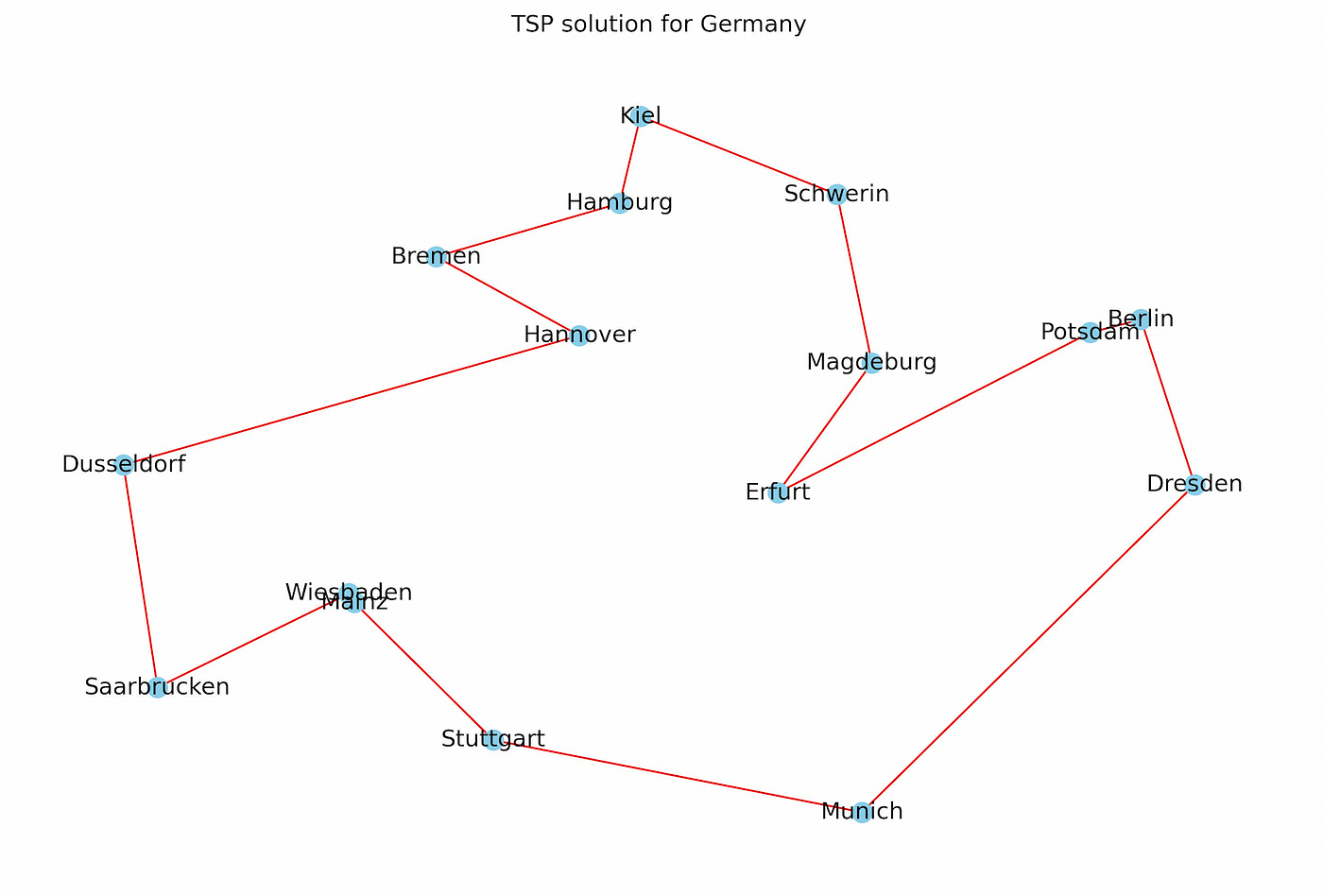
Using the Christofides algorithm as described above, the solution to the TSP is given by cycle. Since cycle consists only of the indices of the cities in capitals, I obtain the solution route indicating the order of cities as tsp_cycle, as given in the screenshot below.
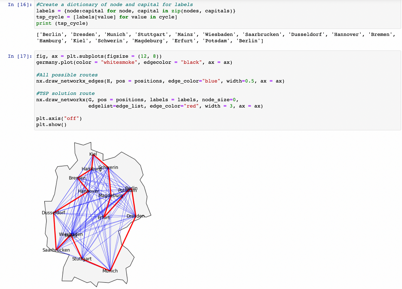
As depicted in In [17] in the screenshot below, I plot the map of Germany with all possible paths between any two cities represented by blue lines. The red lines represent the edge_list, which contains the list of edges between the cities that are part of the solution cycle.
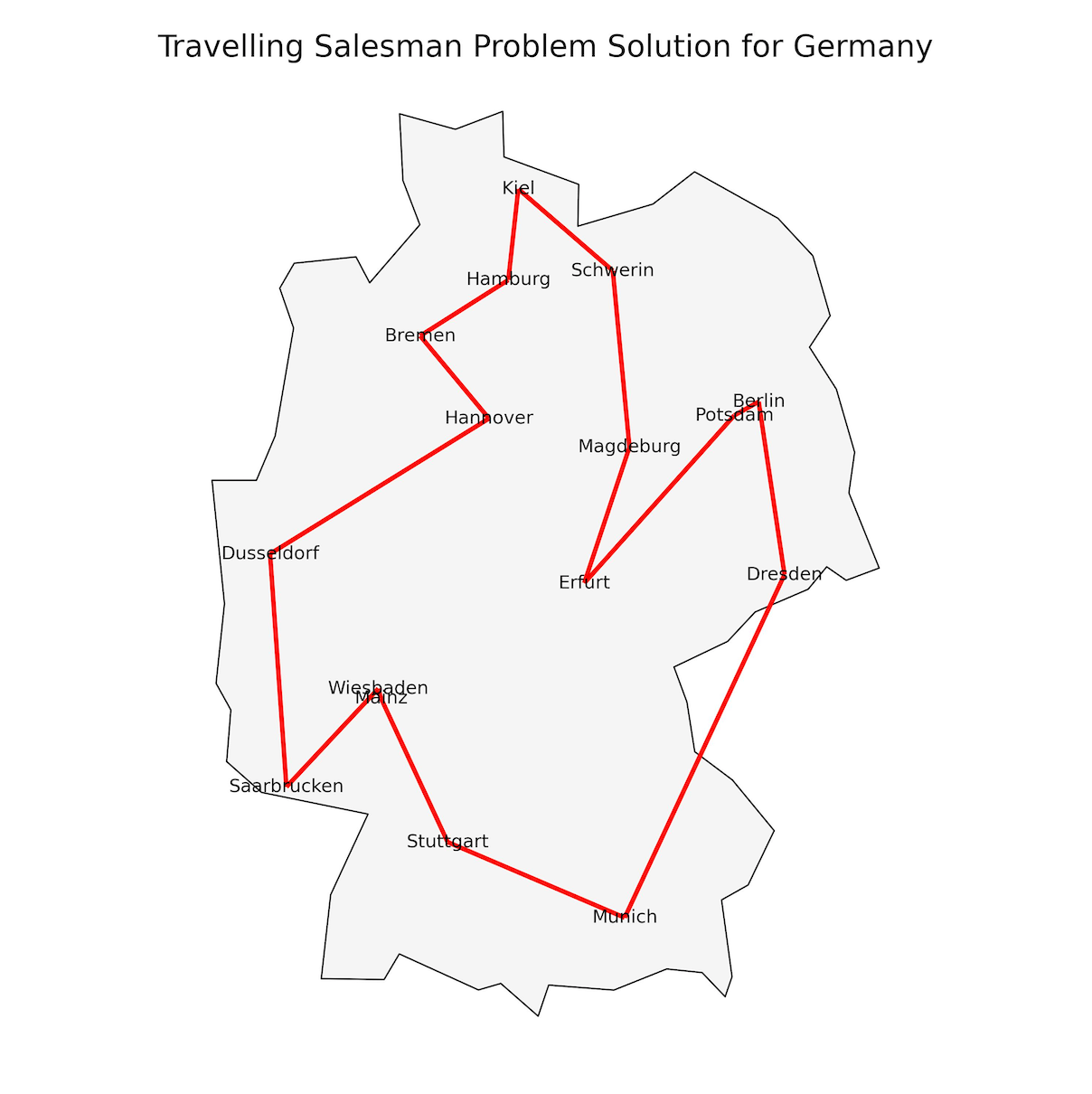
The plot below provides a cleaner solution by removing the blue (all possible) edges between two cities and plotting only the solution to the TSP for Germany in red.
Plotting the solution with unique color for each edge
I wanted to make my solution a bit more attractive by plotting a unique color for each edge between the cities.
Any color used on a computer display can be represented as a proportion of RGB (Red, Green, and Blue) in the visible spectrum (Mathisfun, 2021). Thus, in Python, any color can be represented as #RRGGBB, where RR, GG, and BB have the hexadecimal values ranging from 00 to ff. #000000 represents the white color while #ffffff represents the black color.
I create a function called get_colors(n), which creates a list of random colors based on random values of #RRGGBB in hexadecimal system.
import random
get_colors = lambda n: list(map(lambda i: “#” +”%06x” % random.randint(0, 0xffffff),range(n)))
In the following code, I pass get_colors(16) as the edge_color.
fig, ax = plt.subplots(figsize = (20, 12))germany.plot(ax = ax, color = “whitesmoke”, edgecolor = “black”)# Draw the route
nx.draw_networkx(G, pos = positions, labels = labels,
edgelist=edge_list, edge_color=get_colors(16), width=3,
node_color = “snow”, node_shape = “s”, node_size = 300,
bbox = dict(facecolor = “#ffffff”, boxstyle = “round”,ec = “silver”),
ax = ax)plt.title(“Travelling Salesman Problem Solution for Germany”, fontsize = 15)
plt.axis(“off”)
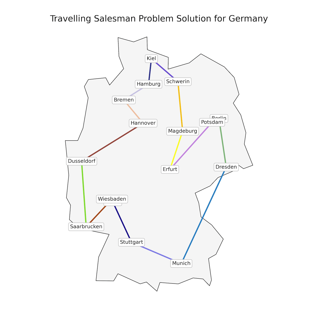
As a result, I get the following plot, which is colorful and more attractive than the previous one along with unique color for each edge in the solution.
Plot solution using folium
The plot above can also be plotted in an interactive leaflet map using the folium package.
For this, I modified the coordinates as folium_coordinates and cycle as route. These are the same data, but in a new format: a list of lists of GPS coordinates (latitude and longitude) to be compatible with folium.
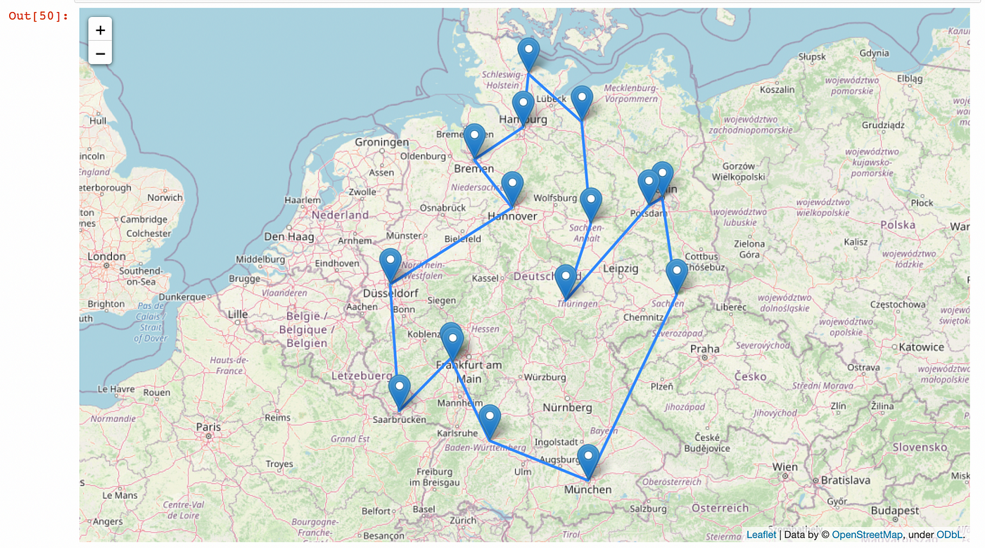
Next, I created a map m1 at location 51°North and 10°East, which is the approximate coordinates for Germany. I choose the OpenStreetMap tiles and zoom_start at 6. I add a marker at the coordinate of each city on the map. And finally, I draw polyline overlays on the map using the route which reflects the solution to the TSP.
The resulting plot is displayed as shown in an interactive leaflet map:
The problem statement of this post was to find the shortest route to travel across the capital cities of 16 federal states of Germany starting in Berlin and ending in Berlin while visiting each city in between exactly once. I started by describing the different complexity classes to solve any decision problem: P (Polynomial-time), NP (Non-deterministic Polynomial-time), and NP-hard. Next, I discussed the concept of Hamilton cycles.
I used geocoding to find the coordinates of the capital cities of 16 federal states of Germany and used the GeoPandas package to plot them on the map of Germany. I added all the edges between any two cities on the map. Next, I demonstrated how the Christofides algorithm provides the solution to the travelling salesman problem through its stepwise implementation. Finally, I plotted a clean solution to this problem using NetworkX, GeoPandas, and Matplotlib packages. I also plotted the solution with a unique color for each edge, as well as plotted the solution in a leaflet package using the folium package.
The implementation of the analyses in this story is available in this GitHub repository. If you want to read further about graph visualisation basics with Python, you can refer to the following story and other accompanying stories in the series.
Thank you for reading!
Bari, 2018. NP-Hard and NP-Complete Problems.
Christofides, 2022. Worst-Case Analysis of a New Heuristics for the Travelling Salesman Problem.
Goodrich and Tamassia, 2014. Algorithm Design and Applications | Wiley
Hayes, 2019. Solving Travelling Salesperson Problems with Python.
Maru, 2020. P, NP, NP Hard and NP Complete Problem | Reduction | NP Hard and NP Compete | Polynomial Class.
Matuszek, 1996. Polynomial-time algorithm.
Mathisfun.com, 2021. Hexadecimal Colours.
Mathworld, 2022a. Hamiltonian Cycle.
Mathworld, 2022b. Perfect Matching.
MIT OpenCourseWare, 2016. R9. Approximation Algorithms: Traveling Salesman Problem
NetworkX, 2015. minimum_spanning_tree.
Tutorialspoint, 2022. Non-Deterministic Turing Machine.
Viswarupan, 2016. P vs NP Problem.
Discovering the shortest route to travel across the capital cities of 16 federal states of Germany while visiting each city once using the Christofides algorithm.
I have been residing in Germany for six years now. Germany is composed of 16 federal states, and I have visited five state capitals until now. Recently, a thought struck my mind:
I want to travel across the capital cities of all 16 federal states and visit each city exactly once while starting in Berlin and ending in Berlin. What would be the shortest possible route to do so?
This type of problem is known as a Travelling Salesman Problem (TSP). As the name suggests, a travelling salesman would go door to door, or region to region within a specified territory trying to sell the products or services of her/his business. The TSP deals with finding the shortest route covering all points exactly once since this would be the most effective route in terms of cost, time, and energy.

A decision problem is a problem having a “Yes” or “No” answer. There could be different complexity classes to solve it. Such as:
- P is a complexity class where the decision problem can be solved in polynomial time by a Deterministic Turing Machine (DTM). A polynomial-time algorithm has an execution time of the order O(nᵏ) for some nonnegative integer k, where n is the complexity of the input.
Problems that can be solved by a polynomial-time algorithm are called tractable problems. Examples of such algorithms are linear search (O(n)), binary search (O(log n)), insertion sort (O(n²)), merge sort (O(n log n)), and matrix multiplication (O(n³)) (Bari, 2018 and Maru, 2020).
- NP (Non-deterministic Polynomial-time) refers to a set of decision problems that can be solved in polynomial-time by a Non-deterministic Turing Machine (NTM). An NTM can have a group of actions to come to the solution, but the transition would be non-deterministic (randomised) for each execution (Tutorialspoint, 2022). Once a potential solution is provided for an NP problem, a DTM can verify its correctness in polynomial time (Viswarupan, 2016).
An algorithm, which is non-deterministic today can also be deterministic if someone finds its solution tomorrow (Bari, 2018 and Maru, 2020). This implies that a problem that can be solved by DTM in polynomial time can also be solved by NTM in polynomial time. Hence, P is a subset of NP.
- NP-hard is the complexity class of decision problems that are “at least as hard as the hardest problem in NP”. A problem H is NP-hard when every problem L in NP can be reduced in polynomial time to H; i.e., assuming a solution for H takes 1 unit time, H’s solution can be used to solve L in polynomial time. The solution of H and L (Yes or No) must also be the same.
TSP is an NP-hard problem. This implies that if there are a large number of cities, it is not feasible to evaluate every possible solution within a “reasonable” time (Hayes, 2019).
To solve the Travelling Salesman Problem (TSP), one needs to first understand the concept of the Hamilton cycle (also referred to as the Hamiltonian cycle). A Hamilton cycle is a graph cycle (closed loop) through a graph that visits each node exactly once (Mathworld, 2022a). This is named after Sir William Rowan Hamilton, who introduced this concept through a game called Hamiltonian puzzle (also known as the Icosian game).
In a graph with n nodes, the total number of possible Hamilton cycles is given by (n-1)! if we consider clockwise and anti-clockwise paths as two different paths. If we consider clockwise and anti-clockwise paths as the same, there are (n-1)!/2 possible Hamilton cycles.
Let’s take an example of four cities: Berlin, Dusseldorf, Hamburg, and Munich. I aim to travel across these four cities starting and ending in Berlin while passing through the cities in between exactly once. The number of possible unique paths (Hamilton cycles) in this example is given by (4–1)! = 3! = 6.
In the code below, cities is a list of these four cities but with start and end as Berlin. The other three cities are defined as *rest. The permutation of these three cities taking all three at a time results in the all possible Hamilton cycles. This is shown in the Python code below.
In the gist below, the make_tsp_tree function first creates a list of Hamilton paths, then creates a directed prefix tree from a list of those paths, and then returns the graph object G by removing the root node and the nil node. The position of each node in G is set using the dot layout of Graphviz, which sets hierarchical structure in directed graphs.
The Hamilton paths for the list of these four cities are presented in the graph below:
I define the list of 16 state capitals of Germany as capitals. Using a process called geocoding, I could get the coordinates of all 16 cities. The process of geocoding using the geopy package is described in detail in this story.
capitals = [‘Berlin’, ‘Bremen’, ‘Dresden’, ‘Dusseldorf’,
‘Erfurt’, ‘Hamburg’, ‘Hannover’, ‘Kiel’,
‘Magdeburg’, ‘Mainz’, ‘Munich’, ‘Potsdam’,   ‘Saarbrucken’, ‘Schwerin’, ‘Stuttgart’, ‘Wiesbaden’]
Using the GeoPandas package, I extract the map of Germany in GeoDataFrame called germany. To plot the capitals in germany, first I create a graph object G using NetworkX. Then I create 16 nodes, one for each city. Next, I create a dictionary of nodes and coordinates of each city for positions. And I create another dictionary of nodes and names of capital cities for labels. The code and the resulting map are given in the screenshot below.
The next step is to determine and plot all the possible paths between any two cities in Germany. Since there are 16 cities in our list, the number of possible paths between any two cities is given by ⁿCᵣ = ¹⁶C₂ = 120. In the existing graph object G, I add the edges between any two nodes except itself as follows:
for i in nodes:
for j in nodes:
if i!=j:
G.add_edge(i, j)
Plotting the updated graph object G with germany with the recently added edges looks as follows:
I create H as a backup copy of G for later use.
Next, I calculate the Euclidean distance between all two cities in Germany, and this information is stored as the weights of the edges in G. Thus, G is now a complete weighted graph in which an edge connects each pair of graph nodes and each edge has a weight associated with it.
H = G.copy()#Calculating the distances between the nodes as edge's weight.
for i in range(len(pos)):
for j in range(i + 1, len(pos)):
#Multidimensional Euclidean distan
dist = math.hypot(pos[i][0] - pos[j][0], pos[i][1] - pos[j][1])
dist = dist
G.add_edge(i, j, weight=dist)
The distance between the cities with each other can be observed in the following table in the matrix format. In the following table, the distance between cities with themselves is zero as observed in the main diagonal. And all the entries above the main diagonal are reflected in the equal entries below the diagonal. Hence, it is an example of a hollow (zero-diagonal) symmetric matrix.
To find the solution cycle, NetworkX uses a default algorithm known as the Christofides algorithm for undirected graphs, and the list of edges that are part of the solution cycle is stored as edge_list. This is implemented in the code below:
cycle = nx_app.christofides(G, weight="weight")
edge_list = list(nx.utils.pairwise(cycle))
Christofides algorithm
The Christofides algorithm finds an approximate solution to the TSP, on instances where the distances form a metric space (they are symmetric and obey the triangle inequality, i.e., in ∆ABC, a+b≥c ) (Goodrich and Tamassia, 2014). This algorithm is named after a Cypriot mathematician named Nicos Christofides, who devised it in 1976. As of now, this algorithm offers the best approximation ratio to solve TSP (Christofides, 2022).
The basic steps of this algorithm are given below. These steps have been implemented in the source code of NetworkX here. I also illustrate the stepwise implementation of the algorithm for our problem.
- Find a minimum (weigh) spanning tree T of G.
The minimum spanning tree for a weighted, connected, undirected graph (here G) is a graph consisting of the subset of edges that together connect all connected nodes (here 16) while minimising the total sum of weights on the edges.
NetworkX uses a Kruskal algorithm to find the minimum spanning tree (NetworkX, 2015). This will look as follows in the case of Germany with the capital cities of its 16 federal states:
2. Make a set of nodes in T with an odd degree O.
In the next step, a set of nodes called O is created in which the degree of each node is odd. From the tree T above, we see that Berlin, Potsdam, Stuttgart, and Schwerin each have degree 2 i.e., even. Therefore, these nodes are removed in the new set O as shown below:
3. Find a minimum-weight perfect matching M in the induced subgraph given by the vertices from O.
To have a perfect matching, there needs to be an even number of nodes in a graph and each node is connected with exactly one other node. A perfect matching is therefore a matching containing n/2 edges (the largest possible) (Mathworld, 2022b).
The minimum weight perfect matching M computes a perfect matching which minimises the weight of matched edges as shown in the plot below.
4. Combine the edges of M and T to form a connected multigraph H.
In the next step, the algorithm combines the edges of T in step 1 with M in step 3 to form a connected multigraph H.
5. Build an Eulerian circuit using the edges of M and T.
In the next step, the Christofides algorithm builds an Eulerian circuit using the edges of M and T. An Eulerian circuit is a trail in a finite graph that visits each edge exactly once. Each node in an Eulerian circuit must have an even degree (MIT OpenCourseWare, 2016). The difference between the Hamilton cycle and the Eulerian cycle is that the Hamilton cycle passes through each node exactly once and ends at the initial node, while the Eulerian cycle passes through each edge exactly once and ends at the initial node.
Note: A cycle can be both a Hamilton cycle and an Eulerian cycle.
6. Convert the Eulerian cycle into a Hamilton cycle by skipping the repeated nodes.
In the case of our TSP, there could be some nodes that are repeated in the Eulerian circuit. Such nodes have a degree of more than 2 i.e., the node is visited more than once. Christofides algorithm utilises a shortcutting function to remove the repeated nodes from the Eulerian circuit and creates a cycle. Thus, the solution to the TSP is achieved by using the list of consecutive edges between the nodes within the cycle.
The weight of the solution produced by Christofides algorithm is within 3/2 of the optimum (MIT OpenCourseWare, 2016).
Using the Christofides algorithm as described above, the solution to the TSP is given by cycle. Since cycle consists only of the indices of the cities in capitals, I obtain the solution route indicating the order of cities as tsp_cycle, as given in the screenshot below.
As depicted in In [17] in the screenshot below, I plot the map of Germany with all possible paths between any two cities represented by blue lines. The red lines represent the edge_list, which contains the list of edges between the cities that are part of the solution cycle.
The plot below provides a cleaner solution by removing the blue (all possible) edges between two cities and plotting only the solution to the TSP for Germany in red.
Plotting the solution with unique color for each edge
I wanted to make my solution a bit more attractive by plotting a unique color for each edge between the cities.
Any color used on a computer display can be represented as a proportion of RGB (Red, Green, and Blue) in the visible spectrum (Mathisfun, 2021). Thus, in Python, any color can be represented as #RRGGBB, where RR, GG, and BB have the hexadecimal values ranging from 00 to ff. #000000 represents the white color while #ffffff represents the black color.
I create a function called get_colors(n), which creates a list of random colors based on random values of #RRGGBB in hexadecimal system.
import random
get_colors = lambda n: list(map(lambda i: “#” +”%06x” % random.randint(0, 0xffffff),range(n)))
In the following code, I pass get_colors(16) as the edge_color.
fig, ax = plt.subplots(figsize = (20, 12))germany.plot(ax = ax, color = “whitesmoke”, edgecolor = “black”)# Draw the route
nx.draw_networkx(G, pos = positions, labels = labels,
edgelist=edge_list, edge_color=get_colors(16), width=3,
node_color = “snow”, node_shape = “s”, node_size = 300,
bbox = dict(facecolor = “#ffffff”, boxstyle = “round”,ec = “silver”),
ax = ax)plt.title(“Travelling Salesman Problem Solution for Germany”, fontsize = 15)
plt.axis(“off”)
As a result, I get the following plot, which is colorful and more attractive than the previous one along with unique color for each edge in the solution.
Plot solution using folium
The plot above can also be plotted in an interactive leaflet map using the folium package.
For this, I modified the coordinates as folium_coordinates and cycle as route. These are the same data, but in a new format: a list of lists of GPS coordinates (latitude and longitude) to be compatible with folium.
Next, I created a map m1 at location 51°North and 10°East, which is the approximate coordinates for Germany. I choose the OpenStreetMap tiles and zoom_start at 6. I add a marker at the coordinate of each city on the map. And finally, I draw polyline overlays on the map using the route which reflects the solution to the TSP.
The resulting plot is displayed as shown in an interactive leaflet map:
The problem statement of this post was to find the shortest route to travel across the capital cities of 16 federal states of Germany starting in Berlin and ending in Berlin while visiting each city in between exactly once. I started by describing the different complexity classes to solve any decision problem: P (Polynomial-time), NP (Non-deterministic Polynomial-time), and NP-hard. Next, I discussed the concept of Hamilton cycles.
I used geocoding to find the coordinates of the capital cities of 16 federal states of Germany and used the GeoPandas package to plot them on the map of Germany. I added all the edges between any two cities on the map. Next, I demonstrated how the Christofides algorithm provides the solution to the travelling salesman problem through its stepwise implementation. Finally, I plotted a clean solution to this problem using NetworkX, GeoPandas, and Matplotlib packages. I also plotted the solution with a unique color for each edge, as well as plotted the solution in a leaflet package using the folium package.
The implementation of the analyses in this story is available in this GitHub repository. If you want to read further about graph visualisation basics with Python, you can refer to the following story and other accompanying stories in the series.
Thank you for reading!
Bari, 2018. NP-Hard and NP-Complete Problems.
Christofides, 2022. Worst-Case Analysis of a New Heuristics for the Travelling Salesman Problem.
Goodrich and Tamassia, 2014. Algorithm Design and Applications | Wiley
Hayes, 2019. Solving Travelling Salesperson Problems with Python.
Maru, 2020. P, NP, NP Hard and NP Complete Problem | Reduction | NP Hard and NP Compete | Polynomial Class.
Matuszek, 1996. Polynomial-time algorithm.
Mathisfun.com, 2021. Hexadecimal Colours.
Mathworld, 2022a. Hamiltonian Cycle.
Mathworld, 2022b. Perfect Matching.
MIT OpenCourseWare, 2016. R9. Approximation Algorithms: Traveling Salesman Problem
NetworkX, 2015. minimum_spanning_tree.
Tutorialspoint, 2022. Non-Deterministic Turing Machine.
Viswarupan, 2016. P vs NP Problem.
Denial of responsibility! Techno Blender is an automatic aggregator of the all world’s media. In each content, the hyperlink to the primary source is specified. All trademarks belong to their rightful owners, all materials to their authors. If you are the owner of the content and do not want us to publish your materials, please contact us by email – [email protected]. The content will be deleted within 24 hours.