
Statistics Bootcamp 4: Bayes, Coins, Fish, Goats, and Cars | by Adrienne Kline | Sep, 2022
Learn the math and methods behind the libraries you use daily as a data scientist
To more formally address the need for a statistics lecture series on Medium, I have started to create a series of statistics boot camps, as seen in the title above. These will build on one another and as such will be numbered accordingly. The motivation for doing so is to democratize the knowledge of statistics in a ground up fashion to address the need for more formal statistics training in the data science community. These will begin simple and expand upwards and outwards, with exercises and worked examples along the way. My personal philosophy when it comes to engineering, coding, and statistics is that if you understand the math and the methods, the abstraction now seen using a multitude of libraries falls away and allows you to be a producer, not only a consumer of information. Many facets of these will be a review for some learners/readers, however having a comprehensive understanding and a resource to refer to is important. Happy reading/learning!
This bootcamp is dedicated to introducing Bayes theorem and doing a deeper dive into some probability distributions.
Bayes’ rule is the rule to compute conditional probability. Some background on Bayes:
- Used to revise probabilities in accordance with newly acquired information
- Derived from the general multiplication rule
- ‘Because this has happened’… ‘This is more or less likely now’ etc.
Supposed that events A1, A2, …Ak are mutually exclusive and exhaustive (as covered in our previous bootcamp). Then for any event B:
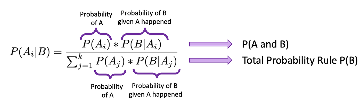
P(A) is the probability of event A when there is no other evidence present, called the prior probability of event A (base rate of A). P(B) is the total probability of happening of event B, and can be subdivided into the denominator in the equation above. P(B) is referred to as the probability of evidence, and derived from the Total Probability Rule. P(B|A) is the probability of happening an event B given that A has occurred, known as the likelihood. P(A|B) is the probability of how likely A happens given that B has already happened. It is known as posterior probability. We are trying to calculate the posterior probability.
What if (from bootcamp 3) in examples of low, medium, and high-risk for stroke and the probability of having a stroke in 5 years, the question was “If a randomly selected subject aged 50 had a stroke in the past 5 years, what is the probability that he/she was in the low-risk group?” Furthermore, you are given the same probabilities as previously (seen below).
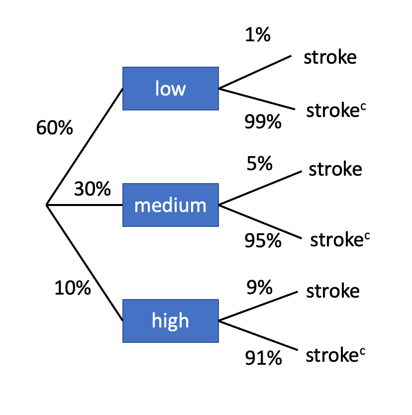
P(low) = 0.6, P(medium) = 0.3, P(high) = 0.1
P(stroke|low) = 0.01, P(stroke|medium) = 0.05, P(stroke|high) = 0.09
P(low|stroke) = ? (this is our posterior probability)

So our answer is if a randomly selected subject aged 50 had a stroke in the past 5 years, what is the probability that he/she was in the low-risk group is 20%.
Let’s think of the classic Monty hall problem. Behind two of these doors, there is a goat, behind the third is your dream car. You select a door. One of the other doors is opened to reveal a goat, not your current selection. Monty asks if you wish to stay with your door or switch to the other door. What should you do? You should switch — but WHY?! Let’s take a look…
When you selected the door the first time you have a 1/3 or 33.33% of selecting correctly (by random) — this is going to change. Let’s say the car is behind door 1 and you picked door 2 …so you are currently in possession of a goat. Monty KNOWS where the car is. He CANNOT open your door OR where the car is. So should you stay or switch? You have just been given 33.33% more so you should switch!
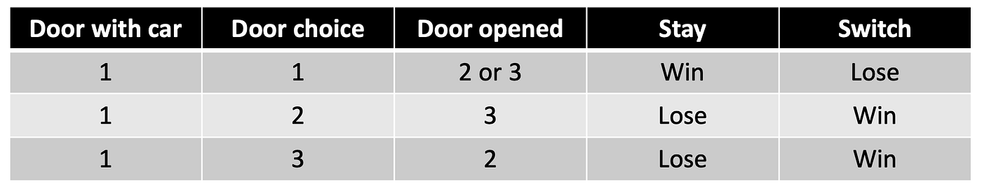
This is why it is a conditional probability problem. We have conditioned on the ‘door opened’ the second time you need to make a decision. If we play this out over all scenarios and all door selections, the same probability holds. If Monty opened a door RANDOMLY your chances of winning the car would be 50% the second time not 66.6% for switching and 33.33% for staying.
Random Variables
A random variable is a quantitative variable whose value depends on chance. Compare this with a discrete random variable, which is a random variable whose possible values can be listed.
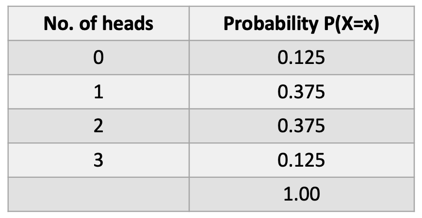
Example. Every day, Jack and Mike stay the latest in the biology lab and toss a coin to decide who will clean up the lab. If it’s heads (H), then Jack will clean up. If it’s tails (T), Mike will do the work. For 3 consecutive days, they report to their lab supervisor. The sample space is:
{H,H,H} {H,H,T} {H,T,T} {T,H,T} {H,T,H} {T,H,H} {T,T,H} {T,T,T}
What is the probability that Jack cleans up the lab 0, 1, 2, or 3 times? (let ‘x’ be the number of times Jack cleans).
Here is the theoretical or expected probability distribution:
Now perform 1000 observations of the random variable X (the number of heads obtained in 3 tosses of a balanced coin). This is the empirical probability distribution (observed).
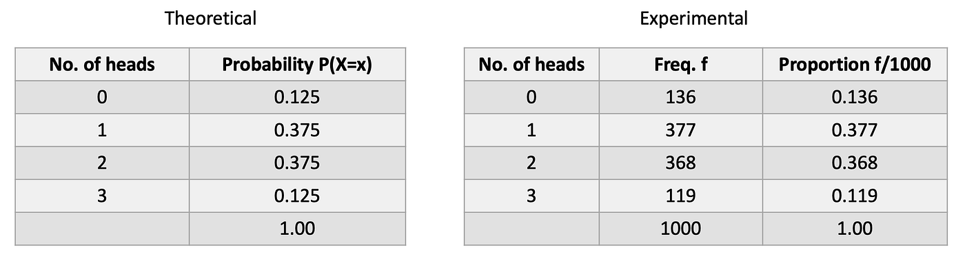
Note that the probabilities in the empirical distribution are fairly close to the probabilities in the theoretical (true) distribution when the number of trials are large.
Law of Large Numbers
If we tossed a balanced coin once, we theorize that there is 50–50 chance the coin will land with heads facing up. What happens if the coin is tossed 50 times? Will head come up exactly 25 times? Not necessarily, due to variation. The law of large numbers states that as the number of trials increases, the empirical probability (estimated probability from observations) will approach the theoretical probability. In this case, 1/2. You can see in the graph below the fraction of heads approaches the theoretical the more tosses are performed.
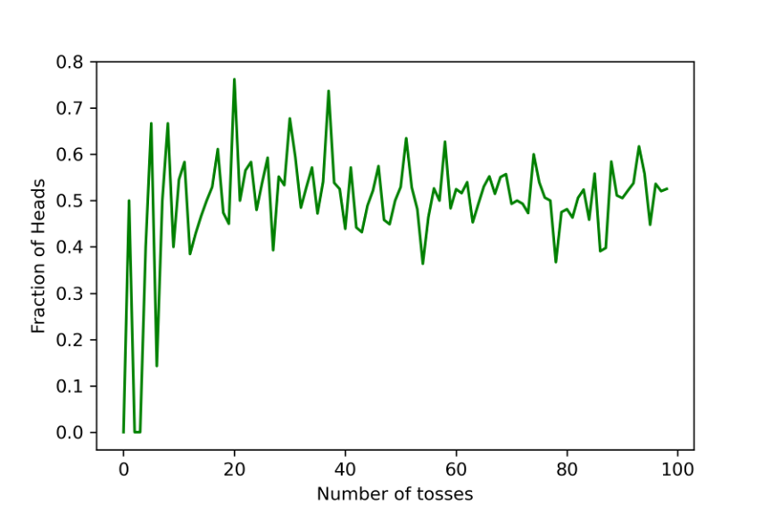
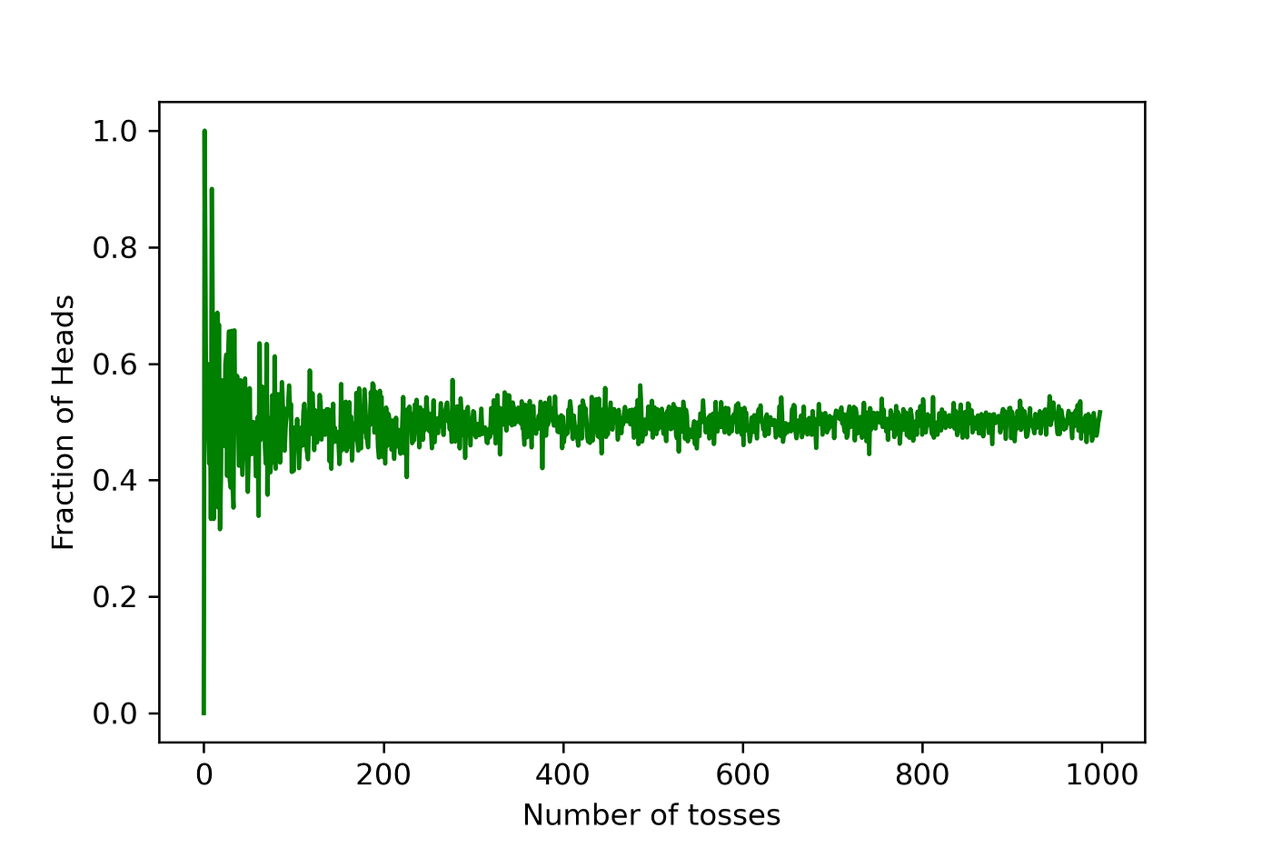
Here is the code to generate the above figure in python:
from random import randint
import matplotlib.pyplot as plt
import numpy as np
import pandas as pd
#num = input('Number of times to flip coin: ')
fracti = []
tosses = []
for num_tosses in range(1,1000):
flips = [randint(0,1) for r in range(int(num_tosses))]
results = []
for object in flips:
if object == 0:
results.append(1)
elif object == 1:
results.append(0)
fracti.append(sum(results)/int(num_tosses))
tosses.append(flips)df = pd.DataFrame(fracti, columns=['toss'])
plt.plot(df['toss'], color='g')
plt.xlabel('Number of tosses')
plt.ylabel('Fraction of Heads')
plt.savefig('toss.png',dpi=300)
Requirements of a probability distribution:
- The sum of the probabilities of a discrete random variable must equal 1, ΣP(X=x)=1.
- The probability of each event in the sample space must be between 0 and 1 (inclusive). I.e. 0≤ P(X) ≤1.
The probability distribution is the same as the relative frequency distribution, however, the relative frequency distribution is empirical and the probability distribution is theoretical.
Discrete Probability Distribution Mean or Expectation
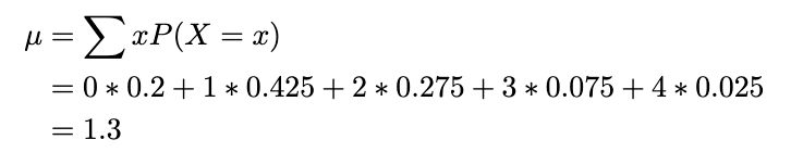
The mean of a discrete random variable X, is denoted μ_x or, when no confusion will arise, simply, μ. it is defined by:
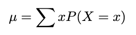
The terms expected value and expectation are commonly used in place of the term mean — and why when you see the capital ‘𝔼’ for expectation, you should think ‘mean’.
To interpret the mean of a random variable, consider a large number of independent observations of a random variable X. The average value of those observation will approximately equal the mean, μ, of X. The larger the number of observations, the closer the average tends to be to μ.
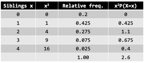
The relative frequency table actually is a discrete probability distribution, which contains random variable (siblings x) and probability of each event (relative frequency). Given the siblings probability distribution in the class, find the expected number (mean) of siblings in this class. The table below shoes the relative frequency distribution.
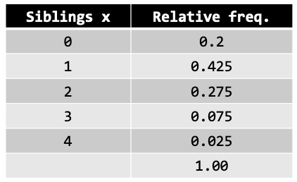
Calculating the mean:
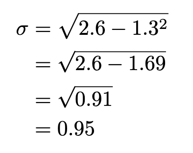
Discrete Probability Distribution Standard Deviations
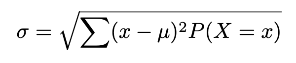
The standard deviation of a discrete random variable X, is denote σ_x, or, when no confusion will arise, simply, σ. It is defined as:
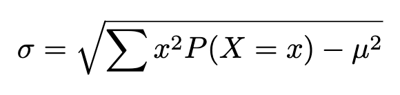
The standard deviation of a discrete random variable can also be obtained from the computing formula:
Performing the operating on our same frequency distribution:
Discrete Probability Distribution Cumulative Probability
Example. Flip a fair coin 10 times. What is the probability of having at most 3 heads?
lets X = total number of heads
P(X≤3)= P(X=0)+P(X=1)+P(X=2)+P(X=3)
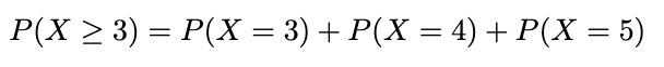
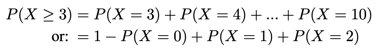
What is the probability of having at least 3 heads?
P(X≥3)= P(X=3)+P(X=4)+P(X=5)+..+P(X=10)
=1- P(X=0)+P(X=1)+P(X=2)
=1-P(X≤2)
What is the probability of having between 2 and 4 (inclusive)?
P(2≤X≤4)= P(X≤4)-P(X<2)
= P(X≤4)-P(X≤1)
= P(X=4)+P(X=3)+P(X=2)
A Bernoulli trial represents an experiment with only 2 possible outcomes (e.g. A and B). The formula is denoted as:
P(X=A) = p, P(X=B) = 1-p=q
p : probability of on the outcomes (e.g. A)
1-p : probability of the other outcome (e.g. B)
Examples:
- flipping a coin
- passing or failing an exam
- assignment of treatment/control group for each subject
- test positive/negative in a screening/diagnostic test
A binomial experiment is the concatenation of several Bernoulli trials. It is a probability experiment that must satisfy the following requirements:
- Must have a fixed number of trials
- Each trial can only have 2 outcomes (e.g. success/failure)
- Trials MUST be independent
- Probability of success must remain the same for each trial
A binomial distribution is a discrete probability distribution of the number of successes in a series of ’n’ independent trials, each having two possible outcomes and a constant probability of success. A Bernoulli distribution can be regarded as a special Binomial distribution when n=1.
Notation:
X~Bin(n,p)
p: probability of success (1-p: probability of failure)
n: number of trails
X: number of success in n trials, with 0≤X≤n
Applying counting rules:
‘X’ successes in ‘n’ trials → p*p*…*p= p^X
n-X: failure → (1-p)*(1-p)*…*(1-p)= (1-p)^(n-X) = q^(n-X)
Binomial Probability Formula (theoretical):
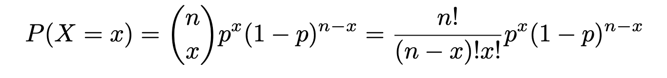
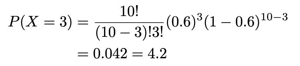
Example. Every day, Adrienne and Banafshe stay the latest in the engineering lab and toss a coin to decide who will clean up the lab. If it’s heads (H), Adrienne will do the work, if tails (T), Banafshe. The coin they used, however, has a 0.7 probability of getting heads. In the following week, find the probability that Adrienne will clean up the lab or exactly 3 days (a week here is the 5 day work week). Let X denote the number of days in a week Adrienne cleans up the lab. X~Bin(5,0.7).
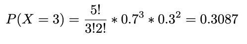
What is the probability that Adrienne will clean up for at least 3 days? We can express it below and go through the same calculation as above adding the probabilities for X=3, X=4, and X=5.
Example. A publication entitled Statistical report on the health of Americans indicated that 3 out of 5 Americans aged 12 years and over visited a physician at least once in the past year. If 10 Americans aged 12+ years are randomly selected, find the probability that exactly 3 people visited a physician at least once last year. Find the probability that at least 3 people visited a physician at least once a year.
n: number of trials=10
X: Number of successed (visited a physician) in n trials = 3
p: numerical probability of success = 3/5
q: numerical probability of failure = 2/5
and:
Mean and Stand. Dev of Binomial Distributions
- mean: μ=n*p
- variance: σ² = n*p*q
- standard deviation: σ= sqrt(n*p*q)
Example. What is the mean and standard deviation of the number of cleaning up Adrienne will do in a week?
n=5, p=0.7, q=0.3
μ = 5*0.7 = 3.5
σ = sqrt(5*0.7*0.3) = 1.02
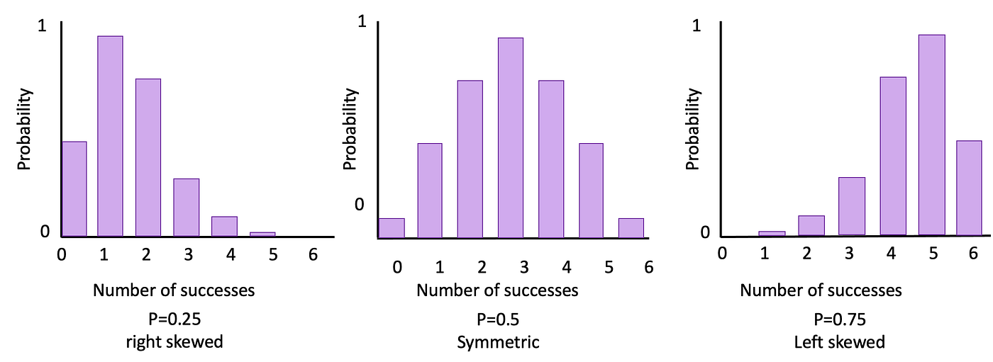
Generally, a binomial distribution is right skewed if p<0.5, is symmetric if p=0.5, and left skewed if p>0.5. The figure below illustrates these facts for 3 different binomial distributions with n=6.
More than 2 outcomes?
What if we have more than two outcomes? Say we’re looking at the M&M’s Cynthia had. We pick 5 with our eyes closed from the box. What is the chance we will have 2 blue, 1 yellow, 1 red and 1 green?
A multinomial distribution is a distribution in which each trial has more than 2 independent outcomes. If X consists of keeping track of k mutually exclusive and exhaustive events E1, E2,..Ek what have corresponding probabilities p1, p2,..pk of occurring, and where X1 is the number of times E1 will occur, X2 is the number of times E2 will occur, etc., then the probability that X (a specific happening of x1, x2, ..) will occur is:
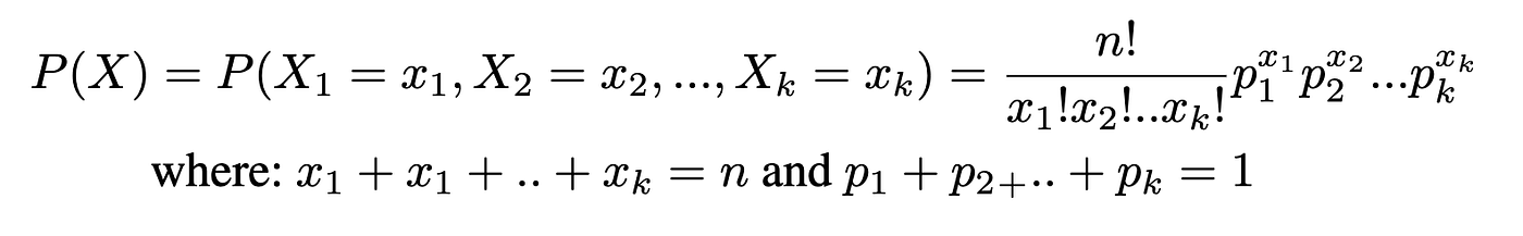
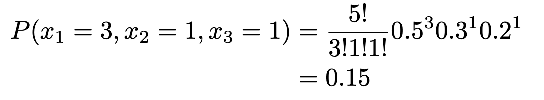
Example. In a large city, 50% of the people choose a movie, 30% choose dinner and a play, and 20% choose shopping, as the most favorable leisure activity. If a sample of 5 people are randomly selected, find the probability that 3 are planning to attend a movie, 1 to a play, and 1 to a shopping mall.
n=5, x1=3, x2=1, x3=1, p1=0.5, p2=0.3, p3=0.2
Now, say we want to plan for avoiding overcrowding in the ER. If we know there are 25,000 visits a year (365 days) at Northwestern Medicine, and the ER handles 60 well a day, what is the chance we will get 68 a day?
Say a bakery will not charge their muffins if they don’t have enough chocolate chips, how could we model this?
The correct pronunciation of Poisson is pwa-sawn, and it means fish in French! A Poisson distribution is a type of discrete probability distribution, that models the frequency with which a specified event occurs during a particular period of time, volume, are etc. (e.g. number of chocolate chips per muffin 😉 ). Formally, it is the probability of X occurrences in an interval (volume, time etc.) for a variable where λ is the mean number of occurrences per unit (time, volume etc.)
The formula is:
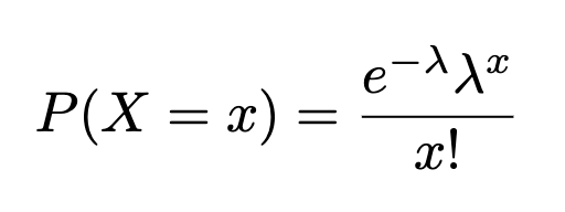
x=0,1,2,…(# of occurrences), e=is the exponential function
- mean: μ = λ
- variance: σ² = λ
- standard deviation: sqrt(λ)
Notice that the mean and the variance are the sam in the Poisson distribution!
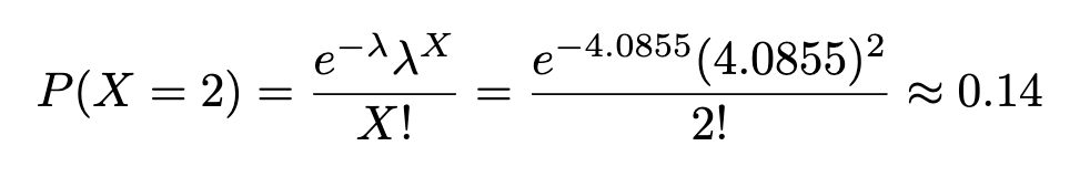
Example. In the black hawks season, 203 injuries were found over 49,687 game hours. Find the probability that 2 injuries occurred within 1000 game hours.
1. Find the injury rate per 1000 game hours
2. X = 2, where X ~ Poisson (λ=4.0855):
Food for thought, literally. Suppose the same bakery as before, has cheap stale croissants and fresh croissants, the newbie at the bakery mixed them all up. There were 14 fresh and 5 stale. If you want to purchase 6 croissants, what are the chances of getting only 1 stale?
A hypergeometric distribution is a distribution of a variable that had two mutually exclusive outcomes when sampling is done WITHOUT replacement. It is usually used when population size is small.
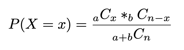
Given a population of two types of objects, such that there are ‘a’ items of type A and ‘b’ items of type B and a+b equals the total population, and we want to choose ’n’ items. What is the probability of selecting ‘x’ number of type A items?
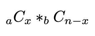
Step 1. The number of ways to select x items of type A (x items from type A, so the rest n-x items must be from type B):
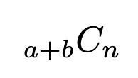
Step 2. The total number of ways to select n items from the pool of (a+b):
So the probability P(X=x) if selecting, without replacement in a sample size of n, X items of type A and n-X items of type B:
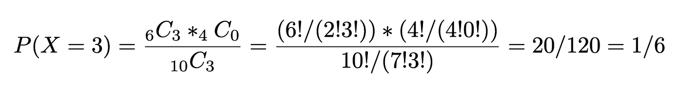
Example. 10 people apply for a position of research coordinator for a basketball study. Six have completed a postgraduate degree and 4 have not. If the investigator of the study selects 3 applicants randomly without replacement, find the probability that all 3 had postgraduate degrees.
a=6 having postgrad degrees
b=4 no postgrad degrees
n=3
X=3
In this bootcamp, we have continued in the vein of probability theory now including work to introduce Bayes theorem and how we can derive it using our previously learned rules of probability (multiplication theory). You have also learned how to think about probability distributions — Poisson, Bernoulli, Multinomial and Hypergeometric. Look out for the next installment of this series, where we will continue to build our knowledge of stats!!
Previous boot camps in the series:
#1 Laying the Foundations
#2 Center, Variation and Position
#3 Probability… Probability
All images unless otherwise stated are created by the author.
Learn the math and methods behind the libraries you use daily as a data scientist

To more formally address the need for a statistics lecture series on Medium, I have started to create a series of statistics boot camps, as seen in the title above. These will build on one another and as such will be numbered accordingly. The motivation for doing so is to democratize the knowledge of statistics in a ground up fashion to address the need for more formal statistics training in the data science community. These will begin simple and expand upwards and outwards, with exercises and worked examples along the way. My personal philosophy when it comes to engineering, coding, and statistics is that if you understand the math and the methods, the abstraction now seen using a multitude of libraries falls away and allows you to be a producer, not only a consumer of information. Many facets of these will be a review for some learners/readers, however having a comprehensive understanding and a resource to refer to is important. Happy reading/learning!
This bootcamp is dedicated to introducing Bayes theorem and doing a deeper dive into some probability distributions.
Bayes’ rule is the rule to compute conditional probability. Some background on Bayes:
- Used to revise probabilities in accordance with newly acquired information
- Derived from the general multiplication rule
- ‘Because this has happened’… ‘This is more or less likely now’ etc.
Supposed that events A1, A2, …Ak are mutually exclusive and exhaustive (as covered in our previous bootcamp). Then for any event B:
P(A) is the probability of event A when there is no other evidence present, called the prior probability of event A (base rate of A). P(B) is the total probability of happening of event B, and can be subdivided into the denominator in the equation above. P(B) is referred to as the probability of evidence, and derived from the Total Probability Rule. P(B|A) is the probability of happening an event B given that A has occurred, known as the likelihood. P(A|B) is the probability of how likely A happens given that B has already happened. It is known as posterior probability. We are trying to calculate the posterior probability.
What if (from bootcamp 3) in examples of low, medium, and high-risk for stroke and the probability of having a stroke in 5 years, the question was “If a randomly selected subject aged 50 had a stroke in the past 5 years, what is the probability that he/she was in the low-risk group?” Furthermore, you are given the same probabilities as previously (seen below).
P(low) = 0.6, P(medium) = 0.3, P(high) = 0.1
P(stroke|low) = 0.01, P(stroke|medium) = 0.05, P(stroke|high) = 0.09
P(low|stroke) = ? (this is our posterior probability)
So our answer is if a randomly selected subject aged 50 had a stroke in the past 5 years, what is the probability that he/she was in the low-risk group is 20%.
Let’s think of the classic Monty hall problem. Behind two of these doors, there is a goat, behind the third is your dream car. You select a door. One of the other doors is opened to reveal a goat, not your current selection. Monty asks if you wish to stay with your door or switch to the other door. What should you do? You should switch — but WHY?! Let’s take a look…
When you selected the door the first time you have a 1/3 or 33.33% of selecting correctly (by random) — this is going to change. Let’s say the car is behind door 1 and you picked door 2 …so you are currently in possession of a goat. Monty KNOWS where the car is. He CANNOT open your door OR where the car is. So should you stay or switch? You have just been given 33.33% more so you should switch!
This is why it is a conditional probability problem. We have conditioned on the ‘door opened’ the second time you need to make a decision. If we play this out over all scenarios and all door selections, the same probability holds. If Monty opened a door RANDOMLY your chances of winning the car would be 50% the second time not 66.6% for switching and 33.33% for staying.
Random Variables
A random variable is a quantitative variable whose value depends on chance. Compare this with a discrete random variable, which is a random variable whose possible values can be listed.
Example. Every day, Jack and Mike stay the latest in the biology lab and toss a coin to decide who will clean up the lab. If it’s heads (H), then Jack will clean up. If it’s tails (T), Mike will do the work. For 3 consecutive days, they report to their lab supervisor. The sample space is:
{H,H,H} {H,H,T} {H,T,T} {T,H,T} {H,T,H} {T,H,H} {T,T,H} {T,T,T}
What is the probability that Jack cleans up the lab 0, 1, 2, or 3 times? (let ‘x’ be the number of times Jack cleans).
Here is the theoretical or expected probability distribution:
Now perform 1000 observations of the random variable X (the number of heads obtained in 3 tosses of a balanced coin). This is the empirical probability distribution (observed).
Note that the probabilities in the empirical distribution are fairly close to the probabilities in the theoretical (true) distribution when the number of trials are large.
Law of Large Numbers
If we tossed a balanced coin once, we theorize that there is 50–50 chance the coin will land with heads facing up. What happens if the coin is tossed 50 times? Will head come up exactly 25 times? Not necessarily, due to variation. The law of large numbers states that as the number of trials increases, the empirical probability (estimated probability from observations) will approach the theoretical probability. In this case, 1/2. You can see in the graph below the fraction of heads approaches the theoretical the more tosses are performed.
Here is the code to generate the above figure in python:
from random import randint
import matplotlib.pyplot as plt
import numpy as np
import pandas as pd
#num = input('Number of times to flip coin: ')
fracti = []
tosses = []
for num_tosses in range(1,1000):
flips = [randint(0,1) for r in range(int(num_tosses))]
results = []
for object in flips:
if object == 0:
results.append(1)
elif object == 1:
results.append(0)
fracti.append(sum(results)/int(num_tosses))
tosses.append(flips)df = pd.DataFrame(fracti, columns=['toss'])
plt.plot(df['toss'], color='g')
plt.xlabel('Number of tosses')
plt.ylabel('Fraction of Heads')
plt.savefig('toss.png',dpi=300)
Requirements of a probability distribution:
- The sum of the probabilities of a discrete random variable must equal 1, ΣP(X=x)=1.
- The probability of each event in the sample space must be between 0 and 1 (inclusive). I.e. 0≤ P(X) ≤1.
The probability distribution is the same as the relative frequency distribution, however, the relative frequency distribution is empirical and the probability distribution is theoretical.
Discrete Probability Distribution Mean or Expectation
The mean of a discrete random variable X, is denoted μ_x or, when no confusion will arise, simply, μ. it is defined by:
The terms expected value and expectation are commonly used in place of the term mean — and why when you see the capital ‘𝔼’ for expectation, you should think ‘mean’.
To interpret the mean of a random variable, consider a large number of independent observations of a random variable X. The average value of those observation will approximately equal the mean, μ, of X. The larger the number of observations, the closer the average tends to be to μ.
The relative frequency table actually is a discrete probability distribution, which contains random variable (siblings x) and probability of each event (relative frequency). Given the siblings probability distribution in the class, find the expected number (mean) of siblings in this class. The table below shoes the relative frequency distribution.
Calculating the mean:
Discrete Probability Distribution Standard Deviations
The standard deviation of a discrete random variable X, is denote σ_x, or, when no confusion will arise, simply, σ. It is defined as:
The standard deviation of a discrete random variable can also be obtained from the computing formula:
Performing the operating on our same frequency distribution:
Discrete Probability Distribution Cumulative Probability
Example. Flip a fair coin 10 times. What is the probability of having at most 3 heads?
lets X = total number of heads
P(X≤3)= P(X=0)+P(X=1)+P(X=2)+P(X=3)
What is the probability of having at least 3 heads?
P(X≥3)= P(X=3)+P(X=4)+P(X=5)+..+P(X=10)
=1- P(X=0)+P(X=1)+P(X=2)
=1-P(X≤2)
What is the probability of having between 2 and 4 (inclusive)?
P(2≤X≤4)= P(X≤4)-P(X<2)
= P(X≤4)-P(X≤1)
= P(X=4)+P(X=3)+P(X=2)
A Bernoulli trial represents an experiment with only 2 possible outcomes (e.g. A and B). The formula is denoted as:
P(X=A) = p, P(X=B) = 1-p=q
p : probability of on the outcomes (e.g. A)
1-p : probability of the other outcome (e.g. B)
Examples:
- flipping a coin
- passing or failing an exam
- assignment of treatment/control group for each subject
- test positive/negative in a screening/diagnostic test
A binomial experiment is the concatenation of several Bernoulli trials. It is a probability experiment that must satisfy the following requirements:
- Must have a fixed number of trials
- Each trial can only have 2 outcomes (e.g. success/failure)
- Trials MUST be independent
- Probability of success must remain the same for each trial
A binomial distribution is a discrete probability distribution of the number of successes in a series of ’n’ independent trials, each having two possible outcomes and a constant probability of success. A Bernoulli distribution can be regarded as a special Binomial distribution when n=1.
Notation:
X~Bin(n,p)
p: probability of success (1-p: probability of failure)
n: number of trails
X: number of success in n trials, with 0≤X≤n
Applying counting rules:
‘X’ successes in ‘n’ trials → p*p*…*p= p^X
n-X: failure → (1-p)*(1-p)*…*(1-p)= (1-p)^(n-X) = q^(n-X)
Binomial Probability Formula (theoretical):
Example. Every day, Adrienne and Banafshe stay the latest in the engineering lab and toss a coin to decide who will clean up the lab. If it’s heads (H), Adrienne will do the work, if tails (T), Banafshe. The coin they used, however, has a 0.7 probability of getting heads. In the following week, find the probability that Adrienne will clean up the lab or exactly 3 days (a week here is the 5 day work week). Let X denote the number of days in a week Adrienne cleans up the lab. X~Bin(5,0.7).
What is the probability that Adrienne will clean up for at least 3 days? We can express it below and go through the same calculation as above adding the probabilities for X=3, X=4, and X=5.
Example. A publication entitled Statistical report on the health of Americans indicated that 3 out of 5 Americans aged 12 years and over visited a physician at least once in the past year. If 10 Americans aged 12+ years are randomly selected, find the probability that exactly 3 people visited a physician at least once last year. Find the probability that at least 3 people visited a physician at least once a year.
n: number of trials=10
X: Number of successed (visited a physician) in n trials = 3
p: numerical probability of success = 3/5
q: numerical probability of failure = 2/5
and:
Mean and Stand. Dev of Binomial Distributions
- mean: μ=n*p
- variance: σ² = n*p*q
- standard deviation: σ= sqrt(n*p*q)
Example. What is the mean and standard deviation of the number of cleaning up Adrienne will do in a week?
n=5, p=0.7, q=0.3
μ = 5*0.7 = 3.5
σ = sqrt(5*0.7*0.3) = 1.02
Generally, a binomial distribution is right skewed if p<0.5, is symmetric if p=0.5, and left skewed if p>0.5. The figure below illustrates these facts for 3 different binomial distributions with n=6.
More than 2 outcomes?
What if we have more than two outcomes? Say we’re looking at the M&M’s Cynthia had. We pick 5 with our eyes closed from the box. What is the chance we will have 2 blue, 1 yellow, 1 red and 1 green?
A multinomial distribution is a distribution in which each trial has more than 2 independent outcomes. If X consists of keeping track of k mutually exclusive and exhaustive events E1, E2,..Ek what have corresponding probabilities p1, p2,..pk of occurring, and where X1 is the number of times E1 will occur, X2 is the number of times E2 will occur, etc., then the probability that X (a specific happening of x1, x2, ..) will occur is:
Example. In a large city, 50% of the people choose a movie, 30% choose dinner and a play, and 20% choose shopping, as the most favorable leisure activity. If a sample of 5 people are randomly selected, find the probability that 3 are planning to attend a movie, 1 to a play, and 1 to a shopping mall.
n=5, x1=3, x2=1, x3=1, p1=0.5, p2=0.3, p3=0.2
Now, say we want to plan for avoiding overcrowding in the ER. If we know there are 25,000 visits a year (365 days) at Northwestern Medicine, and the ER handles 60 well a day, what is the chance we will get 68 a day?
Say a bakery will not charge their muffins if they don’t have enough chocolate chips, how could we model this?
The correct pronunciation of Poisson is pwa-sawn, and it means fish in French! A Poisson distribution is a type of discrete probability distribution, that models the frequency with which a specified event occurs during a particular period of time, volume, are etc. (e.g. number of chocolate chips per muffin 😉 ). Formally, it is the probability of X occurrences in an interval (volume, time etc.) for a variable where λ is the mean number of occurrences per unit (time, volume etc.)
The formula is:
x=0,1,2,…(# of occurrences), e=is the exponential function
- mean: μ = λ
- variance: σ² = λ
- standard deviation: sqrt(λ)
Notice that the mean and the variance are the sam in the Poisson distribution!
Example. In the black hawks season, 203 injuries were found over 49,687 game hours. Find the probability that 2 injuries occurred within 1000 game hours.
1. Find the injury rate per 1000 game hours
2. X = 2, where X ~ Poisson (λ=4.0855):
Food for thought, literally. Suppose the same bakery as before, has cheap stale croissants and fresh croissants, the newbie at the bakery mixed them all up. There were 14 fresh and 5 stale. If you want to purchase 6 croissants, what are the chances of getting only 1 stale?
A hypergeometric distribution is a distribution of a variable that had two mutually exclusive outcomes when sampling is done WITHOUT replacement. It is usually used when population size is small.
Given a population of two types of objects, such that there are ‘a’ items of type A and ‘b’ items of type B and a+b equals the total population, and we want to choose ’n’ items. What is the probability of selecting ‘x’ number of type A items?
Step 1. The number of ways to select x items of type A (x items from type A, so the rest n-x items must be from type B):
Step 2. The total number of ways to select n items from the pool of (a+b):
So the probability P(X=x) if selecting, without replacement in a sample size of n, X items of type A and n-X items of type B:
Example. 10 people apply for a position of research coordinator for a basketball study. Six have completed a postgraduate degree and 4 have not. If the investigator of the study selects 3 applicants randomly without replacement, find the probability that all 3 had postgraduate degrees.
a=6 having postgrad degrees
b=4 no postgrad degrees
n=3
X=3
In this bootcamp, we have continued in the vein of probability theory now including work to introduce Bayes theorem and how we can derive it using our previously learned rules of probability (multiplication theory). You have also learned how to think about probability distributions — Poisson, Bernoulli, Multinomial and Hypergeometric. Look out for the next installment of this series, where we will continue to build our knowledge of stats!!
Previous boot camps in the series:
#1 Laying the Foundations
#2 Center, Variation and Position
#3 Probability… Probability
All images unless otherwise stated are created by the author.
Denial of responsibility! Techno Blender is an automatic aggregator of the all world’s media. In each content, the hyperlink to the primary source is specified. All trademarks belong to their rightful owners, all materials to their authors. If you are the owner of the content and do not want us to publish your materials, please contact us by email – [email protected]. The content will be deleted within 24 hours.