
Survival Analysis for Reliable Forecast Modelling in Production | by Hassan Javed | Jun, 2022
Taking proactive measures to ensure model reliability and availability in production
As businesses increasingly move towards machine learning and analytics based solutions, challenges arise when the models are put into production. One such challenge is the drift in model predictions which makes them less reliable in the long run.
Nowhere is this phenomenon more visible than time series forecast models. Changes in economic cycles, monetary policies, consumer behavior and competitor activity can render the predictions inaccurate.
This problem requires reactive and proactive solutions. A reactive approach to respond to drift in forecast models in production is to set thresholds based on business rules around the forecasts. If the difference between the actual time series and the forecast crosses beyond a specified threshold, it is termed as a drift event and in an automated setting would trigger further analysis or retraining of existing models.
Model reliability and availability
Before we delve deeper into this topic, let’s define a few terms to further our discussion.
Machine learning community refers to the concept of reliability to encompass closely related ideas of uncertainty in model predictions and failures to generalize on production data [1].
In this article, I extend this idea of reliability of predictions as follows:
Model reliability is defined as the reliability of model predictions at a particular point in time.
A reliable model is one whose predictions can be relied upon till we reach a point in time where we might want to replace it. This leads us to the second definition:
Model availability refers to the availability of a model that meets the production requirements of model reliability.
A model that does not meet these requirements should be retrained or replaced.
Comparing Reactive vs Proactive strategies for ensuring model reliability
Reacting to drift events within an automated system seems like a reasonable strategy, if:
- The number of models in production is limited so retraining costs are low.
- The frequency of such events is rare.
- There are no strict requirements on model availability.
With some businesses particularly retail and logistics, the number of time series to be modeled might reach thousands if not hundreds of thousands. Moreover, these time series may be closely related e.g. belonging to the same geography, material and domain etc. Responding to drift events at a large scale with further analysis or retraining of models might chip away significant computational and analysis time.
For a model to be reliable in production with decent uptime before it drifts away and triggers retraining, there must be a strategy in place to foresee model drift in advance. This is so:
- SLA requirements related to model availability can be met.
- Analysis can be done on such cases for root cause analysis in pre-production settings.
- Computational requirements for retraining can be calculated in advance knowing the frequency and prevalence of these events across the models.
It is under the aforementioned circumstances, where a proactive approach might be more suitable. Such an approach should essentially provide a decent estimate of such events even before a model is put into production.
Survival modelling for analyzing forecast model reliability
One approach for estimating model reliability that I have found useful for time series forecast models is to utilize survival analysis to model performance decay in predictive models.
Assuming decent history is available on the model performance or a large number of closely related models are available, we can create a survival model to predict the model decay and do proactive analysis. This analysis will help us quantify computational requirements for retraining and model availability under differenct scenarios and aid in planning in advance.
Here, I’ll demonstrate a simple example whereby we can use a survival model to see what kind of decay is expected from a given set of time series models.
But first, a crash course on survival models.
Survival analysis — A crash course
Survival analysis is a branch of statistics that deals with analyzing time to an event. Survival models predict the time to an event [2]. Examples include the time before equipment failure, time before a loan default etc.
The idea here is to model the survival probability distribution as given below.

Here, T is the waiting time until the occurrence of an event and Survival function is the probability that this waiting time is greater than some time t. In other words, the probability of surviving till time t.
Closely related to survival analysis is the concept of censorship. If we do not know when an event occurs, that event is said to be censored. The most intuitive censorship is when the observation period of our experiment expires and the subject under study does not face an event i.e. it may face an event in the future. Such data is said to be right censored. This is the type of censorship most relevant to our study of model reliability in forecasting.

There are several survival modelling techniques — broadly classified into two categories: namely parametric and non-parametric. Parametric models make assumptions about the form of the survival probability distribution and are good choices when equipped with domain knowledge to back these assumptions. Non-parametric models on the other hand do not make assumptions about the probability distribution and calculate it empirically from the data at hand.
The end goal in both modelling types is to obtain a survival function that given a specified point in time would output the survival probability till that point.
Example Application — M5 forecasting dataset
Now, let’s get down to a concrete example and a proposed solution to the problem of reliability in time series models.
For this example, we’ll take the M5 forecasting dataset. This dataset was used in the 5th iteration of the M-series of forecasting competitions, led by Professor Spyros Makridakis since 1982. The dataset is available here.
The data contains sales at various hierarchical levels i.e. item, department, product categories, and store. It includes stores from three US states i.e. California, Texas, and Wisconsin.
Methodology
In order to conduct this study, we will take some special considerations in two different stages of the pipeline i.e. the preprocessing stage and evaluation metric generation. This evaluation metric in turn will lead to our events and censors.
The design of this experiment has the following configuration. I’ll explain these parameters in detail shortly.
Preprocessing
In preprocessing, based on configuration, we filter the stores and departments in which we are interested. This is followed by melting (wide to long format conversion) of the sales columns into a single column.
The sales data exists at the item level. We sum this up at each store-department level. Now, we have store level sales data for each individual department.
Modelling
We build Prophet models for each store-dept. Prophet is a very popular time series forecasting model developed by Facebook research. We build these models with default parameters and a test forecast horizon of 1 year.
Design for survival analysis

Now, we discuss the crux of the methodology i.e. the steps required to perform survival modelling. There are two utilities for this.
The first utility acts on the test set and calculates MAPE (Mean absolute percentage error — a popular metric to evaluate time series forecasts) on an expanding window starting at week 4 till week 26 (6 months). Why do we calculate MAPE like this?
If we assume that the time to event for a forecasting model in production is the time until its performance degrades beyond a given threshold, we can use survival analysis to model this waiting time and hence take proactive steps to ensure model reliability.
It is by using a metric like expanding window MAPE that produces evaluation scores for a model against time that we can generate time to degradation/decay/drift which in turn can be modelled.
While the first utility generates a time based evaluation metric on the test set, the second utility thresholds the first week at which performance degrades and marks this as an event. The threshold is a MAPE of 10 in configuration. In simple terms, we mark an event on the first week when the expanding MAPE crosses 10. For store-dept models where the threshold isn’t crossed by the end of the study i.e. 26 weeks are marked as censored.
The Kaplan-Meier Estimator
The Kaplan-Meier estimator is a non-parametric estimator of the survival function [3]. It is usually the first baseline model in the survival analysis toolkit. Assuming we have no significant domain knowledge and covariates to inform us, we will use this estimator for the sake of illustration.
The estimator is given by the following formula:

where dᵢ are the events that happened at tᵢ and nᵢ are the total subjects who did not face an event up to tᵢ.
At this stage, we aggregate all observations of events and censors from the store-dept models and build Kaplan-Meier models for each department.
Results
The result of fitting a Kaplan-Meier estimator is a survival function that is plotted here for the duration of our study.
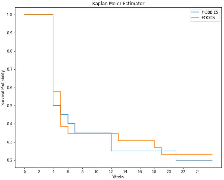
It provides us with the survival probability of models belonging to the Hobbies and Foods departments for each week in our study.
Discussion and interpretation
The probability of survival at the start of the study is 1.0 as expected. The median survival time which is the time at which the probability of survival is 0.5 is 4 weeks for both these departments.
Armed with the survival distribution of our models in production and business rules dictating the probability threshold we can ensure model reliability by taking proactive steps like scheduling retraining and analysis without waiting for a performance incident in production.
An example setup could use the 95th percentile survival time of 2 weeks and retrain all store level models in a given department before this limit is reached in production to ensure that the model degradation is below threshold with the specified probability.
Conclusion
Model availability is facilitated once we take proactive measures like the one described above with survival analysis.
This approach can be performed across models within different categories as well as across modelling strategies for scenarios other than retail and logistics.
Moreover, another aspect that we didn’t touch upon in detail is the fact that this approach requires new metrics for generating time to failure events. These metrics open up a whole lot of opportunities not only for studying model reliability in production but also for serving as individual evaluation metrics based on time, which is very useful for time series forecasting models.
Finally, this article specifically addresses the issues in forecast modelling, but the same principle with appropriate evaluation metrics can be used for other modelling approaches as well.
References
[1] Suchi Saria, Adarsh Subbaswamy, Tutorial: Safe and Reliable Machine Learning (2019), ACM Conference on Fairness, Accountability, and Transparency
[2] Kartsonaki, C., Survival analysis (2016), Diagnostic Histopathology
[3] Jason T. Rich, MD, J. Gail Neel, MD et al, A Practical guide to understanding Kaplan-Meier curves (2014), Otolaryngology–Head and Neck Surgery
[4] Reid, M., Reliability — a Python library for reliability engineering (Version 0.8.2) (2022), https://doi.org/10.5281/ZENODO.3938000
Taking proactive measures to ensure model reliability and availability in production
As businesses increasingly move towards machine learning and analytics based solutions, challenges arise when the models are put into production. One such challenge is the drift in model predictions which makes them less reliable in the long run.
Nowhere is this phenomenon more visible than time series forecast models. Changes in economic cycles, monetary policies, consumer behavior and competitor activity can render the predictions inaccurate.
This problem requires reactive and proactive solutions. A reactive approach to respond to drift in forecast models in production is to set thresholds based on business rules around the forecasts. If the difference between the actual time series and the forecast crosses beyond a specified threshold, it is termed as a drift event and in an automated setting would trigger further analysis or retraining of existing models.
Model reliability and availability
Before we delve deeper into this topic, let’s define a few terms to further our discussion.
Machine learning community refers to the concept of reliability to encompass closely related ideas of uncertainty in model predictions and failures to generalize on production data [1].
In this article, I extend this idea of reliability of predictions as follows:
Model reliability is defined as the reliability of model predictions at a particular point in time.
A reliable model is one whose predictions can be relied upon till we reach a point in time where we might want to replace it. This leads us to the second definition:
Model availability refers to the availability of a model that meets the production requirements of model reliability.
A model that does not meet these requirements should be retrained or replaced.
Comparing Reactive vs Proactive strategies for ensuring model reliability
Reacting to drift events within an automated system seems like a reasonable strategy, if:
- The number of models in production is limited so retraining costs are low.
- The frequency of such events is rare.
- There are no strict requirements on model availability.
With some businesses particularly retail and logistics, the number of time series to be modeled might reach thousands if not hundreds of thousands. Moreover, these time series may be closely related e.g. belonging to the same geography, material and domain etc. Responding to drift events at a large scale with further analysis or retraining of models might chip away significant computational and analysis time.
For a model to be reliable in production with decent uptime before it drifts away and triggers retraining, there must be a strategy in place to foresee model drift in advance. This is so:
- SLA requirements related to model availability can be met.
- Analysis can be done on such cases for root cause analysis in pre-production settings.
- Computational requirements for retraining can be calculated in advance knowing the frequency and prevalence of these events across the models.
It is under the aforementioned circumstances, where a proactive approach might be more suitable. Such an approach should essentially provide a decent estimate of such events even before a model is put into production.
Survival modelling for analyzing forecast model reliability
One approach for estimating model reliability that I have found useful for time series forecast models is to utilize survival analysis to model performance decay in predictive models.
Assuming decent history is available on the model performance or a large number of closely related models are available, we can create a survival model to predict the model decay and do proactive analysis. This analysis will help us quantify computational requirements for retraining and model availability under differenct scenarios and aid in planning in advance.
Here, I’ll demonstrate a simple example whereby we can use a survival model to see what kind of decay is expected from a given set of time series models.
But first, a crash course on survival models.
Survival analysis — A crash course
Survival analysis is a branch of statistics that deals with analyzing time to an event. Survival models predict the time to an event [2]. Examples include the time before equipment failure, time before a loan default etc.
The idea here is to model the survival probability distribution as given below.
Here, T is the waiting time until the occurrence of an event and Survival function is the probability that this waiting time is greater than some time t. In other words, the probability of surviving till time t.
Closely related to survival analysis is the concept of censorship. If we do not know when an event occurs, that event is said to be censored. The most intuitive censorship is when the observation period of our experiment expires and the subject under study does not face an event i.e. it may face an event in the future. Such data is said to be right censored. This is the type of censorship most relevant to our study of model reliability in forecasting.
There are several survival modelling techniques — broadly classified into two categories: namely parametric and non-parametric. Parametric models make assumptions about the form of the survival probability distribution and are good choices when equipped with domain knowledge to back these assumptions. Non-parametric models on the other hand do not make assumptions about the probability distribution and calculate it empirically from the data at hand.
The end goal in both modelling types is to obtain a survival function that given a specified point in time would output the survival probability till that point.
Example Application — M5 forecasting dataset
Now, let’s get down to a concrete example and a proposed solution to the problem of reliability in time series models.
For this example, we’ll take the M5 forecasting dataset. This dataset was used in the 5th iteration of the M-series of forecasting competitions, led by Professor Spyros Makridakis since 1982. The dataset is available here.
The data contains sales at various hierarchical levels i.e. item, department, product categories, and store. It includes stores from three US states i.e. California, Texas, and Wisconsin.
Methodology
In order to conduct this study, we will take some special considerations in two different stages of the pipeline i.e. the preprocessing stage and evaluation metric generation. This evaluation metric in turn will lead to our events and censors.
The design of this experiment has the following configuration. I’ll explain these parameters in detail shortly.
Preprocessing
In preprocessing, based on configuration, we filter the stores and departments in which we are interested. This is followed by melting (wide to long format conversion) of the sales columns into a single column.
The sales data exists at the item level. We sum this up at each store-department level. Now, we have store level sales data for each individual department.
Modelling
We build Prophet models for each store-dept. Prophet is a very popular time series forecasting model developed by Facebook research. We build these models with default parameters and a test forecast horizon of 1 year.
Design for survival analysis
Now, we discuss the crux of the methodology i.e. the steps required to perform survival modelling. There are two utilities for this.
The first utility acts on the test set and calculates MAPE (Mean absolute percentage error — a popular metric to evaluate time series forecasts) on an expanding window starting at week 4 till week 26 (6 months). Why do we calculate MAPE like this?
If we assume that the time to event for a forecasting model in production is the time until its performance degrades beyond a given threshold, we can use survival analysis to model this waiting time and hence take proactive steps to ensure model reliability.
It is by using a metric like expanding window MAPE that produces evaluation scores for a model against time that we can generate time to degradation/decay/drift which in turn can be modelled.
While the first utility generates a time based evaluation metric on the test set, the second utility thresholds the first week at which performance degrades and marks this as an event. The threshold is a MAPE of 10 in configuration. In simple terms, we mark an event on the first week when the expanding MAPE crosses 10. For store-dept models where the threshold isn’t crossed by the end of the study i.e. 26 weeks are marked as censored.
The Kaplan-Meier Estimator
The Kaplan-Meier estimator is a non-parametric estimator of the survival function [3]. It is usually the first baseline model in the survival analysis toolkit. Assuming we have no significant domain knowledge and covariates to inform us, we will use this estimator for the sake of illustration.
The estimator is given by the following formula:
where dᵢ are the events that happened at tᵢ and nᵢ are the total subjects who did not face an event up to tᵢ.
At this stage, we aggregate all observations of events and censors from the store-dept models and build Kaplan-Meier models for each department.
Results
The result of fitting a Kaplan-Meier estimator is a survival function that is plotted here for the duration of our study.
It provides us with the survival probability of models belonging to the Hobbies and Foods departments for each week in our study.
Discussion and interpretation
The probability of survival at the start of the study is 1.0 as expected. The median survival time which is the time at which the probability of survival is 0.5 is 4 weeks for both these departments.
Armed with the survival distribution of our models in production and business rules dictating the probability threshold we can ensure model reliability by taking proactive steps like scheduling retraining and analysis without waiting for a performance incident in production.
An example setup could use the 95th percentile survival time of 2 weeks and retrain all store level models in a given department before this limit is reached in production to ensure that the model degradation is below threshold with the specified probability.
Conclusion
Model availability is facilitated once we take proactive measures like the one described above with survival analysis.
This approach can be performed across models within different categories as well as across modelling strategies for scenarios other than retail and logistics.
Moreover, another aspect that we didn’t touch upon in detail is the fact that this approach requires new metrics for generating time to failure events. These metrics open up a whole lot of opportunities not only for studying model reliability in production but also for serving as individual evaluation metrics based on time, which is very useful for time series forecasting models.
Finally, this article specifically addresses the issues in forecast modelling, but the same principle with appropriate evaluation metrics can be used for other modelling approaches as well.
References
[1] Suchi Saria, Adarsh Subbaswamy, Tutorial: Safe and Reliable Machine Learning (2019), ACM Conference on Fairness, Accountability, and Transparency
[2] Kartsonaki, C., Survival analysis (2016), Diagnostic Histopathology
[3] Jason T. Rich, MD, J. Gail Neel, MD et al, A Practical guide to understanding Kaplan-Meier curves (2014), Otolaryngology–Head and Neck Surgery
[4] Reid, M., Reliability — a Python library for reliability engineering (Version 0.8.2) (2022), https://doi.org/10.5281/ZENODO.3938000
Denial of responsibility! Techno Blender is an automatic aggregator of the all world’s media. In each content, the hyperlink to the primary source is specified. All trademarks belong to their rightful owners, all materials to their authors. If you are the owner of the content and do not want us to publish your materials, please contact us by email – [email protected]. The content will be deleted within 24 hours.