The Bayesian Bootstrap. A short guide to a simple and powerful… | by Matteo Courthoud | Aug, 2022

CAUSAL DATA SCIENCE

A short guide to a simple and powerful alternative to the bootstrap

In causal inference we do not want just to compute treatment effects, we also want to do inference (duh!). In some cases, it’s very easy to compute the (asymptotic) distribution of an estimator, thanks to the central limit theorem. This is the case when computing the average treatment effect in AB tests or randomized controlled trials, for example. However, in other settings, inference is more complicated, when the object of interest is not a sum or an average, as, for example, with the median treatment effect. In these cases, we cannot rely on the central limit theorem. What can we do then?

The bootstrap is the standard answer in data science. It is a very powerful procedure to estimate the distribution of an estimator, without needing any knowledge of the data generating process. It is also very intuitive and simple to implement: just re-sample your data with replacement a lot of times and compute your estimator across samples.

Can we do better? The answer is yes! The Bayesian Bootstrap is a powerful procedure that in a lot of settings performs better than the bootstrap. In particular, it’s usually faster, can give tighter confidence intervals, and avoids a lot of corner cases. In this article, we are going to explore this simple but powerful procedure more in detail.

The bootstrap is a procedure to compute the properties of an estimator by random re-sampling with replacement from the data. It was first introduced by Efron (1979) and it is now a standard inference procedure in data science. The procedure is very simple and consists of the following steps.

Suppose you have access to an i.i.d. sample {Xᵢ}ᵢⁿ and you want to compute a statistic θ using an estimator θ̂(X). You can approximate the distribution of θ̂ as follows.

1. Sample n observations with replacement {X̃ᵢ}ᵢⁿ from your sample {Xᵢ}ᵢⁿ.
2. Compute the estimator θ̂-bootstrap(X̃).
3. Repeat steps 1 and 2 a large number of times.

The distribution of θ̂-bootstrap is a good approximation of the distribution of θ̂.

Why is the bootstrap so powerful?

First of all, it is easy to implement. It does not require you to do anything more than what you were already doing: estimating θ. You just need to do it a lot of times. Indeed, the main disadvantage of the bootstrap is its computational cost. If your estimating procedure is slow, bootstrapping becomes prohibitive.

Second, the bootstrap makes no distributional assumptions. It only assumes that your sample is representative of the population, and observations are independent of each other. This assumption might be violated when observations are tightly connected with each other, such as when studying social networks or market interactions.

Is bootstrap just weighting?

In the end, when we re-sample, what we are doing is assigning integer weights to our observations, such that their sum adds up to the sample size n. Such distribution is the multinomial distribution.

Let’s have a look at what a multinomial distribution looks like by drawing a sample of size 10.000. I import a set of standard libraries and functions from src.utils. I import the code from Deepnote, a Jupyter-like web-based collaborative notebook environment. For our purpose, Deepnote is very handy because it allows me not only to include code but also output, like data and tables.

First of all, we check that indeed the weights sum up to 1000, or equivalently, that we generated a re-sample of the same size of the data.

We can now plot the distribution of weights.

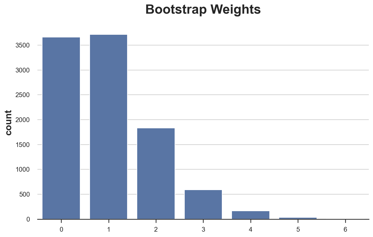
As we can see, around 3600 observations got zero weight, while a couple of observations got a weight of 6. Or equivalently, around 3600 observations did not get re-sampled, while a couple of observations were sampled as many as 6 times.

Now you might have a spontaneous question: why not use continuous weights instead of discrete ones?

Very good question! The Bayesian Bootstrap is the answer.

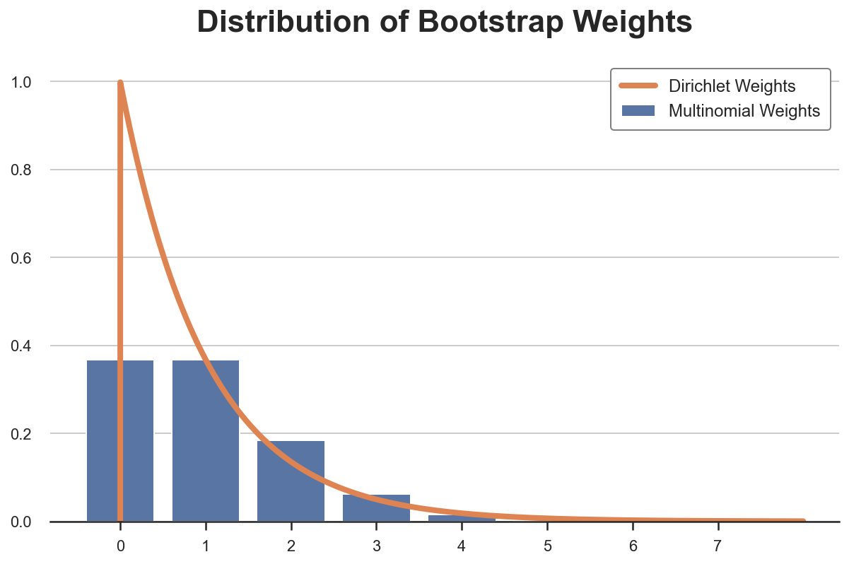
The Bayesian bootstrap was introduced by Rubin (1981) and it’s based on a very simple idea: why not draw a smoother distribution of weights? The continuous equivalent of the multinomial distribution is the Dirichlet distribution. Below I plot the probability distribution of Multinomial and Dirichelet weights for a single observation (they are Poisson and Gamma distributed, respectively).

The Bayesian Bootstrap has many advantages.

• The first and most intuitive one is that it delivers estimates that are much more smooth than the normal bootstrap, because of its continuous weighting scheme.
• Moreover, the continuous weighting scheme prevents corner cases from emerging, since no observation will ever receive zero weight. For example, in linear regression, no problem of collinearity emerges, if there wasn’t one in the original sample.
• Lastly, being a Bayesian method, we gain interpretation: the estimated distribution of the estimator can be interpreted as the posterior distribution with an uninformative prior.

Let’s now draw a set a Dirichlet weights.

The weights naturally sum to (approximately) 1, so we have to scale them by a factor N.

As before, we can plot the distribution of weights, with the difference that now we have continuous weights, so we have to approximate the distribution.

As you might have noticed, the Dirichlet distribution has a parameter α that we have set to 1 for all observations. What does it do?

The α parameter essentially governs both the absolute and relative probability of being sampled. Increasing α for all observations makes the distribution less skewed so that all observations have a more similar weight. For α→∞, all observations receive the same weight and we are back to the original sample.

How should we select the value of α? Shao and Tu (1995) suggest the following.

The distribution of the random weight vector does not have to be restricted to the Diri(l, … , 1). Later investigations found that the weights having a scaled Diri(4, … ,4) distribution give better approximations (Tu and Zheng, 1987)

Let’s have a look at how a Dirichlet distribution with α=4 for all observations compares to our previous distribution with α=1 for all observations.

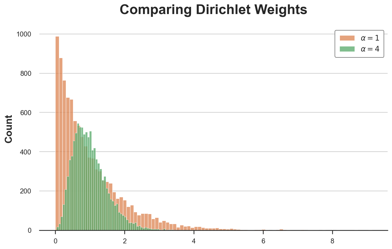
The new distribution is much less skewed and more concentrated around the average value of 1.

Let’s have a look at a couple of examples, where we compare both inference procedures.

Mean of a Skewed Distribution

First, let’s have a look at one of the simplest and most common estimators: the sample mean. First, let’s draw 100 observations from a Pareto distribution.

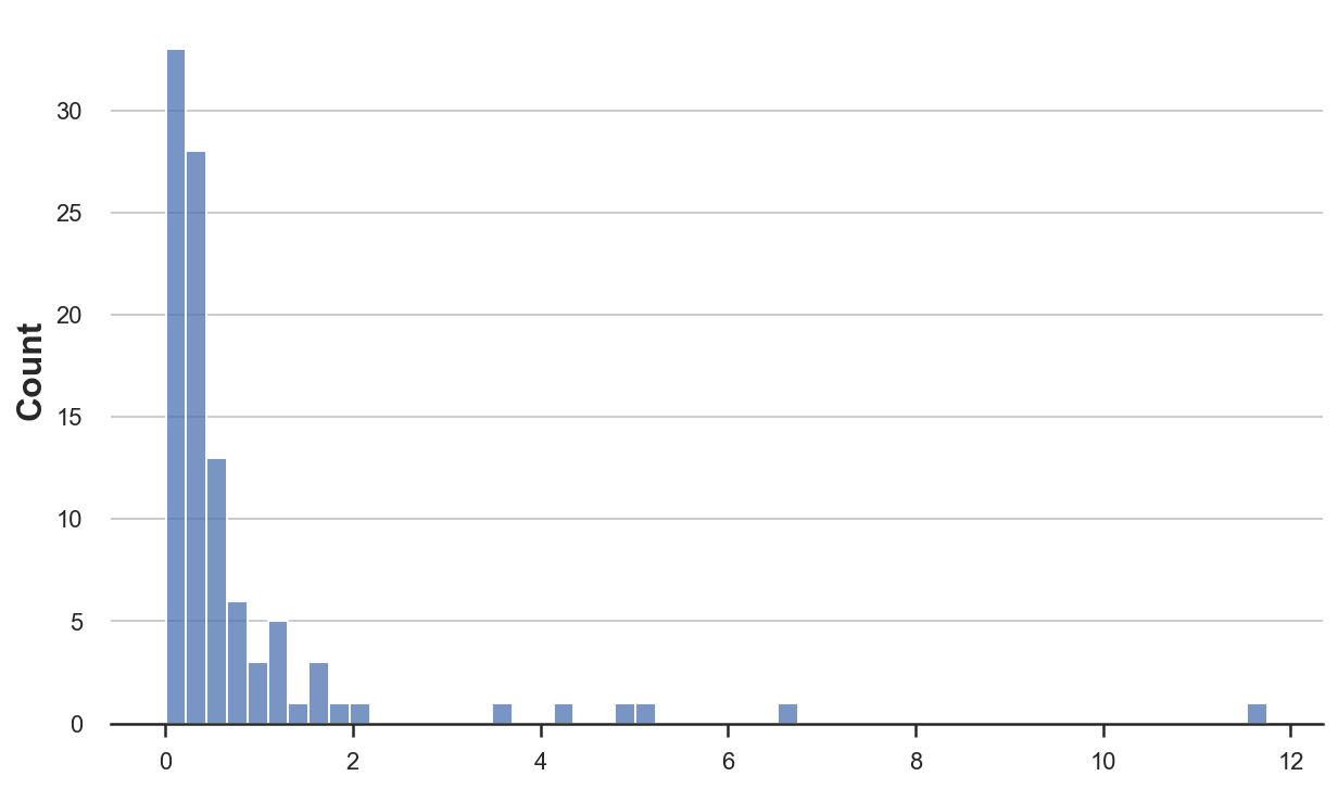
This distribution is very skewed, with a couple of observations taking much higher values than the average.

First, let’s compute the classic bootstrap estimator for one re-sample.

Then, let’s write the Bayesian bootstrap for one set of random weights.

We can now implement any bootstrap procedure. I use the joblib library to parallelize the computation.

Lastly, let’s write a function that compares the results.

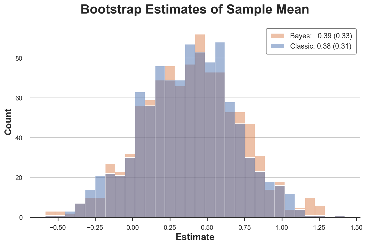
In this setting, both procedures give a very similar answer. The two distributions are very close, and also the estimated mean and standard deviation of the estimator is almost the same, irrespectively to the bootstrap procedure.

Which bootstrap procedure is faster?

The Bayesian bootstrap is faster than the classical bootstrap in 99% of the simulations and by an impressive 75%!

No Weighting? No Problem

What if we have an estimator that does not accept weights, such as the median? We can do two-level sampling: first we sample the weights and then we sample observations according to the weights.

In this setting, the Bayesian Bootstrap is also more precise than the classical bootstrap, because of the denser weight distribution with α=4.

Logistic Regression with Rare Outcome

Let’s now explore the first of two settings in which the classical bootstrap might fall into corner cases. Suppose we observed a feature x, normally distributed, and a binary outcome y. We are interested in the relationship between the two variables.

In this sample, we observe a positive outcome only in 10 observations out of 100.

Since the outcome is binary, we fit a logistic regression model.

We get a point estimate of -23 with a very tight confidence interval.

Can we bootstrap the distribution of our estimator? Let’s try to compute the logistic regression coefficient over 1000 bootstrap samples.

For 5 samples out of 1000, we are unable to compute the estimate. This would not have happened with the Bayesian bootstrap.

This might seem like an innocuous issue in this case: we can just drop those observations. Let’s conclude with a much more dangerous example.

Regression with few Treated Units

Suppose we observed a binary feature x and a continuous outcome y. We are again interested in the relationship between the two variables.

Let’s compare the two bootstrap estimators of the regression coefficient of y on x.

The classic bootstrap procedure estimates a 50% larger variance than our estimator. Why? If we look more closely, we see that in almost 20 re-samples, we get a very unusual estimate of zero! Why?

The problem is that in some samples we might not have any observations with x=1. Therefore, in these re-samples, the estimated coefficient is zero. This does not happen with the Bayesian bootstrap, since it does not drop any observation (all observations always get a positive weight).

The problematic part here is that we are not getting any error message or warning. This bias is very sneaky and could easily go unnoticed!

In this article, we have seen a powerful extension of the bootstrap: the Bayesian bootstrap. The key idea is that whenever our estimator can be expressed as a weighted estimator, the bootstrap is equivalent to random weighting with multinomial weights. The Bayesian bootstrap is equivalent to weighting with Dirichlet weights, the continuous equivalent of the multinomial distribution. Having continuous weights avoids corner cases and can generate a smoother distribution of the estimator.

This article was inspired by the following tweet by Brown University professor Peter Hull.

Indeed, besides being a simple and intuitive procedure, the Bayesian Bootstrap is not part of the standard econometrics curriculum in economic graduate schools.

References

[1] B. Efron Bootstrap Methods: Another Look at the Jackknife (1979), The Annals of Statistics.

[2] D. Rubin, The Bayesian Bootstrap (1981), The Annals of Statistics.

[3] A. Lo, A Large Sample Study of the Bayesian Bootstrap (1987), The Annals of Statistics.

[4] J. Shao, D. Tu, Jacknife and Bootstrap (1995), Springer.

Code

You can find the original Jupyter Notebook here:

Thank you for reading!

I really appreciate it! 🤗 If you liked the post and would like to see more, consider following me. I post once a week on topics related to causal inference and data analysis. I try to keep my posts simple but precise, always providing code, examples, and simulations.

Also, a small disclaimer: I write to learn so mistakes are the norm, even though I try my best. Please, when you spot them, let me know. I also appreciate suggestions on new topics!

CAUSAL DATA SCIENCE

A short guide to a simple and powerful alternative to the bootstrap

In causal inference we do not want just to compute treatment effects, we also want to do inference (duh!). In some cases, it’s very easy to compute the (asymptotic) distribution of an estimator, thanks to the central limit theorem. This is the case when computing the average treatment effect in AB tests or randomized controlled trials, for example. However, in other settings, inference is more complicated, when the object of interest is not a sum or an average, as, for example, with the median treatment effect. In these cases, we cannot rely on the central limit theorem. What can we do then?

The bootstrap is the standard answer in data science. It is a very powerful procedure to estimate the distribution of an estimator, without needing any knowledge of the data generating process. It is also very intuitive and simple to implement: just re-sample your data with replacement a lot of times and compute your estimator across samples.

Can we do better? The answer is yes! The Bayesian Bootstrap is a powerful procedure that in a lot of settings performs better than the bootstrap. In particular, it’s usually faster, can give tighter confidence intervals, and avoids a lot of corner cases. In this article, we are going to explore this simple but powerful procedure more in detail.

The bootstrap is a procedure to compute the properties of an estimator by random re-sampling with replacement from the data. It was first introduced by Efron (1979) and it is now a standard inference procedure in data science. The procedure is very simple and consists of the following steps.

Suppose you have access to an i.i.d. sample {Xᵢ}ᵢⁿ and you want to compute a statistic θ using an estimator θ̂(X). You can approximate the distribution of θ̂ as follows.

1. Sample n observations with replacement {X̃ᵢ}ᵢⁿ from your sample {Xᵢ}ᵢⁿ.
2. Compute the estimator θ̂-bootstrap(X̃).
3. Repeat steps 1 and 2 a large number of times.

The distribution of θ̂-bootstrap is a good approximation of the distribution of θ̂.

Why is the bootstrap so powerful?

First of all, it is easy to implement. It does not require you to do anything more than what you were already doing: estimating θ. You just need to do it a lot of times. Indeed, the main disadvantage of the bootstrap is its computational cost. If your estimating procedure is slow, bootstrapping becomes prohibitive.

Second, the bootstrap makes no distributional assumptions. It only assumes that your sample is representative of the population, and observations are independent of each other. This assumption might be violated when observations are tightly connected with each other, such as when studying social networks or market interactions.

Is bootstrap just weighting?

In the end, when we re-sample, what we are doing is assigning integer weights to our observations, such that their sum adds up to the sample size n. Such distribution is the multinomial distribution.

Let’s have a look at what a multinomial distribution looks like by drawing a sample of size 10.000. I import a set of standard libraries and functions from src.utils. I import the code from Deepnote, a Jupyter-like web-based collaborative notebook environment. For our purpose, Deepnote is very handy because it allows me not only to include code but also output, like data and tables.

First of all, we check that indeed the weights sum up to 1000, or equivalently, that we generated a re-sample of the same size of the data.

We can now plot the distribution of weights.

As we can see, around 3600 observations got zero weight, while a couple of observations got a weight of 6. Or equivalently, around 3600 observations did not get re-sampled, while a couple of observations were sampled as many as 6 times.

Now you might have a spontaneous question: why not use continuous weights instead of discrete ones?

Very good question! The Bayesian Bootstrap is the answer.

The Bayesian bootstrap was introduced by Rubin (1981) and it’s based on a very simple idea: why not draw a smoother distribution of weights? The continuous equivalent of the multinomial distribution is the Dirichlet distribution. Below I plot the probability distribution of Multinomial and Dirichelet weights for a single observation (they are Poisson and Gamma distributed, respectively).

The Bayesian Bootstrap has many advantages.

• The first and most intuitive one is that it delivers estimates that are much more smooth than the normal bootstrap, because of its continuous weighting scheme.
• Moreover, the continuous weighting scheme prevents corner cases from emerging, since no observation will ever receive zero weight. For example, in linear regression, no problem of collinearity emerges, if there wasn’t one in the original sample.
• Lastly, being a Bayesian method, we gain interpretation: the estimated distribution of the estimator can be interpreted as the posterior distribution with an uninformative prior.

Let’s now draw a set a Dirichlet weights.

The weights naturally sum to (approximately) 1, so we have to scale them by a factor N.

As before, we can plot the distribution of weights, with the difference that now we have continuous weights, so we have to approximate the distribution.

As you might have noticed, the Dirichlet distribution has a parameter α that we have set to 1 for all observations. What does it do?

The α parameter essentially governs both the absolute and relative probability of being sampled. Increasing α for all observations makes the distribution less skewed so that all observations have a more similar weight. For α→∞, all observations receive the same weight and we are back to the original sample.

How should we select the value of α? Shao and Tu (1995) suggest the following.

The distribution of the random weight vector does not have to be restricted to the Diri(l, … , 1). Later investigations found that the weights having a scaled Diri(4, … ,4) distribution give better approximations (Tu and Zheng, 1987)

Let’s have a look at how a Dirichlet distribution with α=4 for all observations compares to our previous distribution with α=1 for all observations.

The new distribution is much less skewed and more concentrated around the average value of 1.

Let’s have a look at a couple of examples, where we compare both inference procedures.

Mean of a Skewed Distribution

First, let’s have a look at one of the simplest and most common estimators: the sample mean. First, let’s draw 100 observations from a Pareto distribution.

This distribution is very skewed, with a couple of observations taking much higher values than the average.

First, let’s compute the classic bootstrap estimator for one re-sample.

Then, let’s write the Bayesian bootstrap for one set of random weights.

We can now implement any bootstrap procedure. I use the joblib library to parallelize the computation.

Lastly, let’s write a function that compares the results.

In this setting, both procedures give a very similar answer. The two distributions are very close, and also the estimated mean and standard deviation of the estimator is almost the same, irrespectively to the bootstrap procedure.

Which bootstrap procedure is faster?

The Bayesian bootstrap is faster than the classical bootstrap in 99% of the simulations and by an impressive 75%!

No Weighting? No Problem

What if we have an estimator that does not accept weights, such as the median? We can do two-level sampling: first we sample the weights and then we sample observations according to the weights.

In this setting, the Bayesian Bootstrap is also more precise than the classical bootstrap, because of the denser weight distribution with α=4.

Logistic Regression with Rare Outcome

Let’s now explore the first of two settings in which the classical bootstrap might fall into corner cases. Suppose we observed a feature x, normally distributed, and a binary outcome y. We are interested in the relationship between the two variables.

In this sample, we observe a positive outcome only in 10 observations out of 100.

Since the outcome is binary, we fit a logistic regression model.

We get a point estimate of -23 with a very tight confidence interval.

Can we bootstrap the distribution of our estimator? Let’s try to compute the logistic regression coefficient over 1000 bootstrap samples.

For 5 samples out of 1000, we are unable to compute the estimate. This would not have happened with the Bayesian bootstrap.

This might seem like an innocuous issue in this case: we can just drop those observations. Let’s conclude with a much more dangerous example.

Regression with few Treated Units

Suppose we observed a binary feature x and a continuous outcome y. We are again interested in the relationship between the two variables.

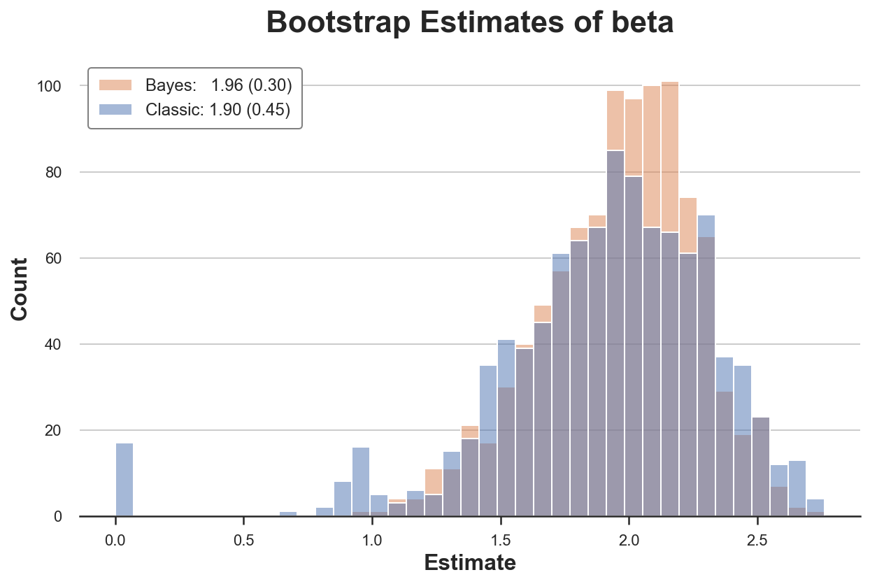
Let’s compare the two bootstrap estimators of the regression coefficient of y on x.

The classic bootstrap procedure estimates a 50% larger variance than our estimator. Why? If we look more closely, we see that in almost 20 re-samples, we get a very unusual estimate of zero! Why?

The problem is that in some samples we might not have any observations with x=1. Therefore, in these re-samples, the estimated coefficient is zero. This does not happen with the Bayesian bootstrap, since it does not drop any observation (all observations always get a positive weight).

The problematic part here is that we are not getting any error message or warning. This bias is very sneaky and could easily go unnoticed!

In this article, we have seen a powerful extension of the bootstrap: the Bayesian bootstrap. The key idea is that whenever our estimator can be expressed as a weighted estimator, the bootstrap is equivalent to random weighting with multinomial weights. The Bayesian bootstrap is equivalent to weighting with Dirichlet weights, the continuous equivalent of the multinomial distribution. Having continuous weights avoids corner cases and can generate a smoother distribution of the estimator.

This article was inspired by the following tweet by Brown University professor Peter Hull.

Indeed, besides being a simple and intuitive procedure, the Bayesian Bootstrap is not part of the standard econometrics curriculum in economic graduate schools.

References

[1] B. Efron Bootstrap Methods: Another Look at the Jackknife (1979), The Annals of Statistics.

[2] D. Rubin, The Bayesian Bootstrap (1981), The Annals of Statistics.

[3] A. Lo, A Large Sample Study of the Bayesian Bootstrap (1987), The Annals of Statistics.

[4] J. Shao, D. Tu, Jacknife and Bootstrap (1995), Springer.

Code

You can find the original Jupyter Notebook here:

Thank you for reading!

I really appreciate it! 🤗 If you liked the post and would like to see more, consider following me. I post once a week on topics related to causal inference and data analysis. I try to keep my posts simple but precise, always providing code, examples, and simulations.

Also, a small disclaimer: I write to learn so mistakes are the norm, even though I try my best. Please, when you spot them, let me know. I also appreciate suggestions on new topics!