
The inductive bias of ML models, and why you should care about it | by Gleb Kumichev | Jun, 2022
What inductive bias is, and how it can harm or help your models
Imagine it’s your first time in Switzerland, you hike in mountains and come across a cow with spots and a cowbell.
You may assume that all spotted caws in Switzerland have a cowbell. This is a typical example of inductive reasoning. It starts with an observation (a cow with spots and a cowbell) and leads to a possible generalization hypothesis (all caws with spots have a cowbell).
Notice that it is possible to draw (induce) other hypotheses based on the same observation. For example, there are cows in Switzerland, all cows have a cowbell regardless of having spots, there are only cows in Switzerland, etc. As one can see, it is possible to make a dozen of hypotheses based on a single observation — this is an important property of inductive reasoning: valid observation may lead to different hypotheses and some of them can be false.

So how can one choose a single hypothesis? To do it, one can choose the simplest hypothesis which is “there are cows in Switzerland”. It can be treated as simple as it has no extra constraints on spots or cowbells, it is just a simple generalization. Such an approach is called “Occam’s razor” and can be treated as one of the simplest inductive biases — choose the simplest hypothesis that describes an observation.
Occam’s razor principle derived from philosophical perspective but also has an equivalent mathematical statement, for example Solomonoff’s theory of inductive inference.
So how does it relate to machine learning?
In most machine learning tasks, we deal with some subset of observations (samples) and our goal is to create a generalization based on them. We also want our generalization to be valid for new unseen data. In other words, we want to draw a general rule that works for the whole population of samples based on a limited sample subset.
So we have some set of observations and a set of hypotheses that can be induced based on observations. The set of observations is our data and the set of hypotheses are ML algorithms with all the possible parameters that can be learned from this data. Each model can describe training data but provide significantly different results on new unseen data.

There is an infinite set of hypotheses for a finite set of samples. For example, consider observations of two points of some single-variable function. It is possible to fit a single linear model and an infinite amount of periodic or polynomial functions that perfectly fit the observations. Given the data, all of that functions are valid hypotheses that perfectly align with observations, and with no additional assumptions, choosing one over another is like making a random guess.

Now let’s infer our hypothesis from the new unseen data sample X2, and it turns out that most of the complicated functions are inaccurate. However, the linear function appears to be quite accurate, which may seem already familiar to you from a bias-variance tradeoff perspective.

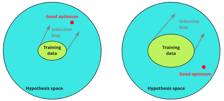
The prioritization of some hypotheses (restriction of hypothesis space) is an inductive bias. So the model is biased toward some group of hypotheses. For the previous example, one can choose a linear model based on some prior knowledge about data and thus prioritize linear generalization.
Why should one care?
As one can see from the previous example, choosing the right induction bias of the model leads to better generalization, especially in a low data setting. The less training data we have, the stronger inductive bias should be to help the model to generalize well. But in a rich data setting, it may be preferable to avoid any induction bias to let the model be less constrained and search through the hypothesis space freely.
How do we choose a model given the task at hand? Usually, the answer is something like this: use CNN for images, use RNN for sequential data, etc. At the same time, it is possible to use RNN for images, CNN for sequential data, etc. The reason to prefer first is the inductive bias of models that are suitable for data. Choosing a model with the right bias boosts chances of finding a better generalization with less data, and that is always desirable. It may be tempting to think that there is some optimal bias that always helps the model to generalize well, but it is impossible to find such a bias according to the “no free launch” theorem. That is why, for every particular problem, we should use specific algorithms and biases.
In the following section, we’ll consider some basic and well-known inductive biases for different algorithms and some less-known examples as well.
Regression models
Probably the most straightforward example is the inductive bias of the regression models that find a solution to a specific equation. Such bias constrains hypothesis space to a single family of equations and optimizes only their coefficients. Such an approach works well in low data settings, especially when one has prior knowledge about functional relations in data, for example, when dealing with data from physics experiments or fitting specific probability distribution.

Additional inductive biases can be injected with regularizations, such as L1 or L2 regularization, for example. They also reduce hypothesis space, adding constraints on model weights. The correct choice of regularization should reflect prior knowledge of the data.
Decision trees
In the decision tree, one of the main inductive biases is the assumption that an objective can be achieved by asking a series of binary questions. As a result, the decision boundary of the tree classifier becomes orthogonal.

It is possible to decrease inductive bias when using random forests and rotational trees that may lead to smoother, more flexible decision boundaries.
Bayesian models
In Bayesian models, one can include prior knowledge or assumptions in the model with prior distribution. This is the same as the injection of specific induction bias. Consider the estimation of a probability of a coin landing heads up: let r be the probability of landing heads up, and Ynbe the number of heads in ntrials.

It is possible to estimate posterior landing heads up probability p(r|Yn) using Binomial distribution for likelihood p(Yn|r) and Betta distribution for prior p(r).

Consider the example with different Betta priors where the ground truth probability of a coin landing heads up is 0.7. If a prior distribution is far from the ground truth, one needs more samples to get closer to the true value estimation.

Convolutional Neural Networks (CNNs)
CNNs have biases that are architecture-specific and biases that mostly depend on data and training procedure. Most general CNNs inductive biases are a locality and weight sharing. Locality implies that closely placed pixels are related to each other. Weight sharing implies searching for specific patterns. Different parts of an image should be processed in the same way. Two more inductive biases are usually implemented into CNNs: translation invariance with pooling layers and translation equivariance without them being used.
Less obvious inductive biases of CNNs are now well-studied and have quite an interesting history. In [1] authors conduct experiments on the triplets of images with shape-match and color-match in a one-shot learning setup and figure out a shape bias of CNN models, which means they rely more on object shape rather than on object color. One year later [2] other researchers argue that there is no shape bias in CNN’s by design and that CNN can be trained to classify shape with proper initialization and data augmentation. Then another research [3] shows that ImageNet trained models are texture-biased.

Authors argue that this type of bias is induced by the dataset rather than by model architecture, and show that they can achieve shape-based representation during training on a stylized dataset that replaces original image textures.
In [4] authors conclude that it is possible to achieve texture bias or shape bias in CNN’s models. The bias is mostly defined by the data and its augmentation procedure, rather than the model architecture itself. They show that data augmentation, such as color distortion or blur, decreases texture bias, whereas random-crop increases it. Finally, researchers [5] show that texture and shape biases are complementary and the model can be trained unbiasedly, equally relying on both texture and shape. To achieve this, the model was trained on a dataset with conflicting shape and texture images (texture from one class and shape from another).

Such an approach improves the recognition model accuracy and robustness of the models.
Those CNN examples reveal the importance of inductive bias. The model can be trained with either biases towards the texture or biases towards the shape, depending on the training procedure and data. Both cases may be equal in terms of accuracy on a test set, but the shape-based model will be more robust against noise corruption and image distortions.
Recurrent Neural Networks (RNNs)
Recurrent neural networks have several architectural biases:
- sequential bias — input tokens processed sequentially one by one (may be reduced by bidirectional RNNs).
- memory bottleneck — a model has no access to past tokens until it processes the first tokens into a hidden state.
- recursion — a model applies the same function for all input data at every step.
Plane RNN also has a locality bias that is reduced in recurrent architectures with longer sequence memorization mechanisms, such as LSTM or GRU.
In the NLP field, research shows that, for some tasks, RNN induction bias may be beneficial. For example, in [8] authors show that LSTM is superior to plane transformers in subject-verb agreement task. It also shows that transformers performance can be gained with RNN inductive bias injections, such as sequential bias (by future token masking) and recurrent bias (by parameters sharing across layers).

Other research shows that LSTM-based models have a bias toward hierarchical induction [9].

Such a hierarchical bias is believed to be useful for NLP tasks.
Transformers
Transformers have no strong inductive biases, so they are more flexible and more data-hungry models. Absence of strong bias puts no additional constraints on a model. As a result, it can find better optimum if enough data is provided. The drawback is that such models perform worse in a low data setting. Injection of some bias may be profitable even for transformers. For example, in computer vision [7] authors proposed to use “soft” convolution inductive bias so that their model can learn to ignore it if necessary. A model can benefit from convolution inductive bias in low data setting and being able to ignore it if it put too much constrains.

Such bias is implemented via Gated Positional Self-Attention layers that can control convolutional inductive bias with learning parameter alpha. Such a model outperforms DeiT and appears to be more sample-efficient. Authors also show that the earliest layers tend to use convolutional inductive bias (alpha is nonzero) and the latest layers tend to ignore the bias altogether (alpha is close to zero).
In [6] authors show that vision transformer models such as ViT or Swin and MLP-mixer models have more shape bias than CNN models.
Graph Neural Networks (GNNs)
GNNs have a strong relation bias. Because of the graph structure, the model strongly relies on structural relations between objects. It is a useful bias for modelling discrete data that can be represented as objects and relations, for example documents database, atoms in molecule or double pendulum, etc.
GNNs are also have permutation invariance bias that is also a desirable property for data with arbitrary ordering. In Graph Convolution Networks there is also weights sharing (as in CNNs), so different parts of the graph are processed in a same way.
Conclusion
Inductive bias can be treated as the initial beliefs about the model and the data properties. Right initial beliefs lead to better generalization with less data. Wrong beliefs may constrain a model too much and will ultimately prevent one from finding a good optimum, even with tons of data. The rule of thumb is to choose models with strong inductive bias, if the desirable bias is clear, and to choose more flexible models with more data, if the desirable bias is not clear.
Every component of the training pipeline, from model initialization and data augmentation to an optimizer or even scheduler, has its own biases that affect a final optimum. Moreover, deep neural network models also have hidden and unknown biases, which is a relevant area of research. Practitioners should also be aware of possible hidden biases that may lead to unexpected model behaviour in the case of data corruption or domain shift.
What inductive bias is, and how it can harm or help your models
Imagine it’s your first time in Switzerland, you hike in mountains and come across a cow with spots and a cowbell.

You may assume that all spotted caws in Switzerland have a cowbell. This is a typical example of inductive reasoning. It starts with an observation (a cow with spots and a cowbell) and leads to a possible generalization hypothesis (all caws with spots have a cowbell).
Notice that it is possible to draw (induce) other hypotheses based on the same observation. For example, there are cows in Switzerland, all cows have a cowbell regardless of having spots, there are only cows in Switzerland, etc. As one can see, it is possible to make a dozen of hypotheses based on a single observation — this is an important property of inductive reasoning: valid observation may lead to different hypotheses and some of them can be false.
So how can one choose a single hypothesis? To do it, one can choose the simplest hypothesis which is “there are cows in Switzerland”. It can be treated as simple as it has no extra constraints on spots or cowbells, it is just a simple generalization. Such an approach is called “Occam’s razor” and can be treated as one of the simplest inductive biases — choose the simplest hypothesis that describes an observation.
Occam’s razor principle derived from philosophical perspective but also has an equivalent mathematical statement, for example Solomonoff’s theory of inductive inference.
So how does it relate to machine learning?
In most machine learning tasks, we deal with some subset of observations (samples) and our goal is to create a generalization based on them. We also want our generalization to be valid for new unseen data. In other words, we want to draw a general rule that works for the whole population of samples based on a limited sample subset.
So we have some set of observations and a set of hypotheses that can be induced based on observations. The set of observations is our data and the set of hypotheses are ML algorithms with all the possible parameters that can be learned from this data. Each model can describe training data but provide significantly different results on new unseen data.
There is an infinite set of hypotheses for a finite set of samples. For example, consider observations of two points of some single-variable function. It is possible to fit a single linear model and an infinite amount of periodic or polynomial functions that perfectly fit the observations. Given the data, all of that functions are valid hypotheses that perfectly align with observations, and with no additional assumptions, choosing one over another is like making a random guess.
Now let’s infer our hypothesis from the new unseen data sample X2, and it turns out that most of the complicated functions are inaccurate. However, the linear function appears to be quite accurate, which may seem already familiar to you from a bias-variance tradeoff perspective.
The prioritization of some hypotheses (restriction of hypothesis space) is an inductive bias. So the model is biased toward some group of hypotheses. For the previous example, one can choose a linear model based on some prior knowledge about data and thus prioritize linear generalization.
Why should one care?
As one can see from the previous example, choosing the right induction bias of the model leads to better generalization, especially in a low data setting. The less training data we have, the stronger inductive bias should be to help the model to generalize well. But in a rich data setting, it may be preferable to avoid any induction bias to let the model be less constrained and search through the hypothesis space freely.
How do we choose a model given the task at hand? Usually, the answer is something like this: use CNN for images, use RNN for sequential data, etc. At the same time, it is possible to use RNN for images, CNN for sequential data, etc. The reason to prefer first is the inductive bias of models that are suitable for data. Choosing a model with the right bias boosts chances of finding a better generalization with less data, and that is always desirable. It may be tempting to think that there is some optimal bias that always helps the model to generalize well, but it is impossible to find such a bias according to the “no free launch” theorem. That is why, for every particular problem, we should use specific algorithms and biases.
In the following section, we’ll consider some basic and well-known inductive biases for different algorithms and some less-known examples as well.
Regression models
Probably the most straightforward example is the inductive bias of the regression models that find a solution to a specific equation. Such bias constrains hypothesis space to a single family of equations and optimizes only their coefficients. Such an approach works well in low data settings, especially when one has prior knowledge about functional relations in data, for example, when dealing with data from physics experiments or fitting specific probability distribution.
Additional inductive biases can be injected with regularizations, such as L1 or L2 regularization, for example. They also reduce hypothesis space, adding constraints on model weights. The correct choice of regularization should reflect prior knowledge of the data.
Decision trees
In the decision tree, one of the main inductive biases is the assumption that an objective can be achieved by asking a series of binary questions. As a result, the decision boundary of the tree classifier becomes orthogonal.
It is possible to decrease inductive bias when using random forests and rotational trees that may lead to smoother, more flexible decision boundaries.
Bayesian models
In Bayesian models, one can include prior knowledge or assumptions in the model with prior distribution. This is the same as the injection of specific induction bias. Consider the estimation of a probability of a coin landing heads up: let r be the probability of landing heads up, and Ynbe the number of heads in ntrials.
It is possible to estimate posterior landing heads up probability p(r|Yn) using Binomial distribution for likelihood p(Yn|r) and Betta distribution for prior p(r).
Consider the example with different Betta priors where the ground truth probability of a coin landing heads up is 0.7. If a prior distribution is far from the ground truth, one needs more samples to get closer to the true value estimation.
Convolutional Neural Networks (CNNs)
CNNs have biases that are architecture-specific and biases that mostly depend on data and training procedure. Most general CNNs inductive biases are a locality and weight sharing. Locality implies that closely placed pixels are related to each other. Weight sharing implies searching for specific patterns. Different parts of an image should be processed in the same way. Two more inductive biases are usually implemented into CNNs: translation invariance with pooling layers and translation equivariance without them being used.
Less obvious inductive biases of CNNs are now well-studied and have quite an interesting history. In [1] authors conduct experiments on the triplets of images with shape-match and color-match in a one-shot learning setup and figure out a shape bias of CNN models, which means they rely more on object shape rather than on object color. One year later [2] other researchers argue that there is no shape bias in CNN’s by design and that CNN can be trained to classify shape with proper initialization and data augmentation. Then another research [3] shows that ImageNet trained models are texture-biased.
Authors argue that this type of bias is induced by the dataset rather than by model architecture, and show that they can achieve shape-based representation during training on a stylized dataset that replaces original image textures.
In [4] authors conclude that it is possible to achieve texture bias or shape bias in CNN’s models. The bias is mostly defined by the data and its augmentation procedure, rather than the model architecture itself. They show that data augmentation, such as color distortion or blur, decreases texture bias, whereas random-crop increases it. Finally, researchers [5] show that texture and shape biases are complementary and the model can be trained unbiasedly, equally relying on both texture and shape. To achieve this, the model was trained on a dataset with conflicting shape and texture images (texture from one class and shape from another).
Such an approach improves the recognition model accuracy and robustness of the models.
Those CNN examples reveal the importance of inductive bias. The model can be trained with either biases towards the texture or biases towards the shape, depending on the training procedure and data. Both cases may be equal in terms of accuracy on a test set, but the shape-based model will be more robust against noise corruption and image distortions.
Recurrent Neural Networks (RNNs)
Recurrent neural networks have several architectural biases:
- sequential bias — input tokens processed sequentially one by one (may be reduced by bidirectional RNNs).
- memory bottleneck — a model has no access to past tokens until it processes the first tokens into a hidden state.
- recursion — a model applies the same function for all input data at every step.
Plane RNN also has a locality bias that is reduced in recurrent architectures with longer sequence memorization mechanisms, such as LSTM or GRU.
In the NLP field, research shows that, for some tasks, RNN induction bias may be beneficial. For example, in [8] authors show that LSTM is superior to plane transformers in subject-verb agreement task. It also shows that transformers performance can be gained with RNN inductive bias injections, such as sequential bias (by future token masking) and recurrent bias (by parameters sharing across layers).
Other research shows that LSTM-based models have a bias toward hierarchical induction [9].
Such a hierarchical bias is believed to be useful for NLP tasks.
Transformers
Transformers have no strong inductive biases, so they are more flexible and more data-hungry models. Absence of strong bias puts no additional constraints on a model. As a result, it can find better optimum if enough data is provided. The drawback is that such models perform worse in a low data setting. Injection of some bias may be profitable even for transformers. For example, in computer vision [7] authors proposed to use “soft” convolution inductive bias so that their model can learn to ignore it if necessary. A model can benefit from convolution inductive bias in low data setting and being able to ignore it if it put too much constrains.
Such bias is implemented via Gated Positional Self-Attention layers that can control convolutional inductive bias with learning parameter alpha. Such a model outperforms DeiT and appears to be more sample-efficient. Authors also show that the earliest layers tend to use convolutional inductive bias (alpha is nonzero) and the latest layers tend to ignore the bias altogether (alpha is close to zero).
In [6] authors show that vision transformer models such as ViT or Swin and MLP-mixer models have more shape bias than CNN models.
Graph Neural Networks (GNNs)
GNNs have a strong relation bias. Because of the graph structure, the model strongly relies on structural relations between objects. It is a useful bias for modelling discrete data that can be represented as objects and relations, for example documents database, atoms in molecule or double pendulum, etc.
GNNs are also have permutation invariance bias that is also a desirable property for data with arbitrary ordering. In Graph Convolution Networks there is also weights sharing (as in CNNs), so different parts of the graph are processed in a same way.
Conclusion
Inductive bias can be treated as the initial beliefs about the model and the data properties. Right initial beliefs lead to better generalization with less data. Wrong beliefs may constrain a model too much and will ultimately prevent one from finding a good optimum, even with tons of data. The rule of thumb is to choose models with strong inductive bias, if the desirable bias is clear, and to choose more flexible models with more data, if the desirable bias is not clear.
Every component of the training pipeline, from model initialization and data augmentation to an optimizer or even scheduler, has its own biases that affect a final optimum. Moreover, deep neural network models also have hidden and unknown biases, which is a relevant area of research. Practitioners should also be aware of possible hidden biases that may lead to unexpected model behaviour in the case of data corruption or domain shift.
Denial of responsibility! Techno Blender is an automatic aggregator of the all world’s media. In each content, the hyperlink to the primary source is specified. All trademarks belong to their rightful owners, all materials to their authors. If you are the owner of the content and do not want us to publish your materials, please contact us by email – [email protected]. The content will be deleted within 24 hours.