The Reasonable Effectiveness of Deep Learning for Time Series Forecasting | by Gabriele Orlandi | Jun, 2022

By Jessie Hobb On Jun 25, 2022

Building blocks for state-of-the-art models

When talking about Time Series, people often tend to do it in a very practical data-oriented way: if you try and look up some definition, you may find expressions such as “a series of data points indexed (or listed or graphed) in time order” (Wikipedia), “a set of data collected at successive points in time or over successive periods of time” (Encyclopædia Britannica), “a sequence of data points that occur in successive order over some period of time” (Investopedia).

Truth is, really everything that can be measured falls under this category; as soon as we start paying attention and observe a phenomenon for more than one snapshot, we can legitimately deal with it with the established theory of Time Series modeling.

The only quantities I can think of that don’t make sense as Time Series are the fundamental physical constants: the good old speed of light c, the gravitational constant G, the fundamental electric charge e… guys like them really never change, at all.

I want to spend a couple more sentences on this because I need to drive a point home: we cannot talk about Time Series and tools for dealing with them under the pretence of completeness.

Indeed, each Time Series is nothing but a single realization of a specific, possibly very complex physical process, with its own possibly infinite set of potential stochastic outcomes.

Realizing the vastness of possibilities should help us tone down our desire to find a one-size-fits-all solution for the tasks of characterizing, classifying or forecasting Time Series.

Examples of Time Series showing just how different their look and their generating process can be [1].

In short, forecasting is the task of predicting future values of a target Time Series based on its past values, values of other related series and features correlating the series to each other.

We usually denote by Y the target series, and use X for its covariates; of course, this is arbitrary since all series we use will be, at least in principle, covariates to each other.

It is instead a meaningful distinction to denote by another letter, say Z, those Time Series with known future values: think calendar features, such as week numbers and holidays.

These series can help at inference as well as during training, and must be treated differently from the others: for one thing, they do not require forecasting.

Another naming convention worth mentioning relates to time: the series start at a conventional initial time t=0, then we use T to denote the split between past (t=0 to T) and future (t>T), or training and testing; h indicates the forecasting horizon, i.e. how many time units in the future we need the forecast to reach (t=T+1 to t=T+h).

Finally, to account for different subgroups and relations across all covariates, forecasting models often allow for the specification of so-called static features (W); these are nothing more than values labeling each series.

For example, we might have a set of series representing household consumption of electricity, whose static features describe the households themselves (number of occupants, house size and so on).

Basic classification of objects used in forecasting.

Notice in the picture that every object is denoted in bold, which is usually reserved for vectors: this is because, a priori, one can also deal with series having more than one value for each time step.

We call such multiple-valued series multi-variate, as opposed to the more common uni-variate series. Here we are borrowing from the statistical jargon: in statistics, a multi-variate probability distribution is one that depends on more than one random variable.

Classification

Whenever we have to face a forecasting problem, we can immediately start to shed some light on it by giving it some labels; for this, we can keep in mind the following classification, based on the definitions we gave so far:

Data-driven criteria

Availability of covariates or static features.
Dimension of the data point: uni- or multi-variate.

Problem-driven criteria

Forecast type, point or probabilistic (quantiles).
Horizon size, i.e. number of predicted time steps in one pass.

Time Series forecasting is an established field, in which an arsenal of statistical tools and theories had already been known before the advent of more contemporary Machine Learning techniques. We won’t focus too much on these, but it is nonetheless useful to run through the most common ones.

Baselines

The first thing that comes to mind when thinking about future values of something surely is to look at its current value; on second thought, one would definitely look at past values as well, and settle for an average or maybe try and follow a trend.

So-called “simple” forecasting methods [1].

We call these methods simple; they are conceptually important because they already tell us that having asymmetric data (the arrow of time going forward, versus the uniformity of e.g. tabular data where every sample gets treated the same way) adds a level of complexity, requiring us to make some assumptions:

Will the future look like now?
Does it matter what the past looked like? How far back should we look?
Is the process underneath the outcomes the same as it was before and as it will be later?

If the answers to these questions are all “yes”, i.e. we assume that all past information is useful and there is a single pattern to follow, we resort to regression methods to find the best function to approximate our data, by searching among increasingly complex families: linear, polynomial, splines, etc.

Unless we know for some reason about some preferred family of functions to search into, we will just pick the optimal function with respect to data. This, though, again stems a few doubts:

Do we expect the more recent trends to continue indefinitely?
Will past peaks and valleys happen again?
Does it even make sense for the series to reach those values that regression predicts for the future?

Decomposition methods

It should be clear now that we cannot rely on data alone, we need at least come contextual information on the process that generates it.

Decomposition methods go in this direction, being most useful when we know that the series comes from a process having some sort of periodicity.

In the most classic of these methods, the Season-Trend-Remainder decomposition, we look for a slow-changing smooth baseline (trend), then turn to fast repeating components (seasonalities), and finally we treat the rest of the signal as random noise (remainder).

STR decomposition forecasting method [1].

Decomposition methods give us more freedom for using our knowledge about data to forecast its future: for example, in tourism-related data we may expect to find weekly (weekends) or yearly (summers) patterns: encoding these periodicities into the model reassures us that forecasts will be less “dumb” and more “informed”.

SARIMAX methods

Finally for this overview of classical forecasting methods, SARIMAX methods are an even more flexible framework allowing to select components that best approximate the Time Series.

The letters making the SARIMAX acronym represent analytical blocks that we can compose together into the equations of the model:

Seasonal if the Time Series has a periodic component;
(Vector) if the Time Series is multivariate;
Auto-Regressive if the Time Series depends on its previous values;
Integrated if the Time Series is non-stationary (e.g. it has a trend);
Moving Average if the Time Series depends on previous forecast errors;
eXogenous variables if there are covariates to exploit.

SARIMAX models have been incredibly successful while being conceptually quite simple, and best represent how one should deal with a forecasting problem: use all information you have about the problem to restrict the class of models to search into, then look for the best approximation of your data lying inside that class.

Many recent review papers [2][3][4] have outlined how, after a too long period of general lack of interest from practitioners, Machine Learning models and especially Neural Networks are becoming ever more central in the Time Series forecasting discourse.

To understand why Deep Learning in particular is especially suited for this problem, we shall tie a conceptual thread that links classical techniques to the most recent and successful architectures.

Training a (dense) neural network, in a nutshell.

The reasonable effectiveness of Deep Learning

As it stands, we know that many types of Neural Network are universal approximators of any (reasonably defined) function, provided they are fed with enough data and memory [5][6][7].

This of course makes them an excellent candidate for any supervised learning problem, where the goal is indeed to learn a function that satisfies known input-output associations.

Sadly, though, theoretical properties like universal approximation often fail to be relevant in practice, where the theorem hypotheses do not hold: in particular, we never have enough data and memory to successfully perform a learning task with any generic universal architecture.

There is though another weapon in Neural Networks’ arsenal, and that is the possibility of injecting information about a problem a priori, in a way that helps the model learn the desired function as if we had more data or computational time to spend.

We can do this by configuring the architecture of the network, i.e. by designing particular network connectivity and shape depending on the problem at hand: this amounts to essentially constraining the search space of possible functions and imposing a computational flow that results in optimal parameters of the network.

From this idea, and years of research in this direction, a taxonomy of network structures and the related problem they effectively solve is being compiled; the approach is somewhat artisanal and heuristic at times, but generalizing and elegant mathematical theories are emerging as well [8].

From a generic dense network to a highly complex one (TFT) [10].

The key advantage of Deep Learning is not, then, its universality, but rather its versatility and modularity: the ability to easily play with a network by extending it, composing it, and rewiring its nodes is crucial for finding the right candidate model for a specific problem.

Moreover, when such model has been found, modularity can streamline the transition to similar problems without losing all acquired expertise (see transfer learning).

All of these features make Deep Learning the perfect successor to classical techniques, continuing the trend of growing model complexity and specialization but also bringing huge boosts in universality and versatility.

Contemporary DL architectures such as N-BEATS [9] are modular and composable.

We are only now getting to understand how shaping a Neural Network’s architecture changes the classes of functions it approximates best, but it is clear that tailoring it to a specific class of problems by imposing a certain shape and structure is immensely beneficial: indeed, this practice has the advantage of pointing the network towards the right direction from the start, thus reducing the time and resources spent on wrong paths.

Now, what are the most useful ingredients for building Deep Learning models that can tackle the hardest forecasting problems?

As we said before, each forecasting problem requires its recipe; it is therefore instructive to look at a few selected network structures and see how they address specific features of the problem by shaping the computational flow and the resulting trained model.

The same nodes can become different blocks when rewired appropriately [15].

Please note that we will only give a very concise description of the architectures we’re going to talk about, and then only focus on how they address learning specific features of a Time Series.

Unsurprisingly, there are many resources out there covering the more technical and mathematical details; for example, Dive Into Deep Learning [15] is very comprehensive and should cover all basic concepts and definitions.

Convolutional Neural Networks

Convolutional networks, or CNNs, have been around for quite a long time and proved successful for many supervised learning tasks.

Their most striking achievement is learning image features, such as classifying pictures based on whether something specific is depicted inside of them.

More generally, a CNN is useful whenever our data at hand:

can be meaningfully represented in tensor form: 1D array, 2D matrix…,
contains meaningful patterns in points that are close to each other in the tensor, but independently of where in the tensor they are.

It’s easy to see how image classification suits this technique:

pictures are naturally matrices of pixels, and
the classification is usually based on the presence of an object inside of it, which is depicted as a group of adjacent pixels.

Note that the “meaningfulness” depends on the problem we are trying to solve, since patterns and representations may make sense only for certain goals.

For example, consider the problem of correctly assigning famous paintings to their painter, or the art movement they belong to: it is not obvious that patterns of adjacent pixels can help with classification, since for example detecting an object can be useful for some (renaissance artists did a lot of portraits), but not for others (how would it help with more contemporary genres?) [16].

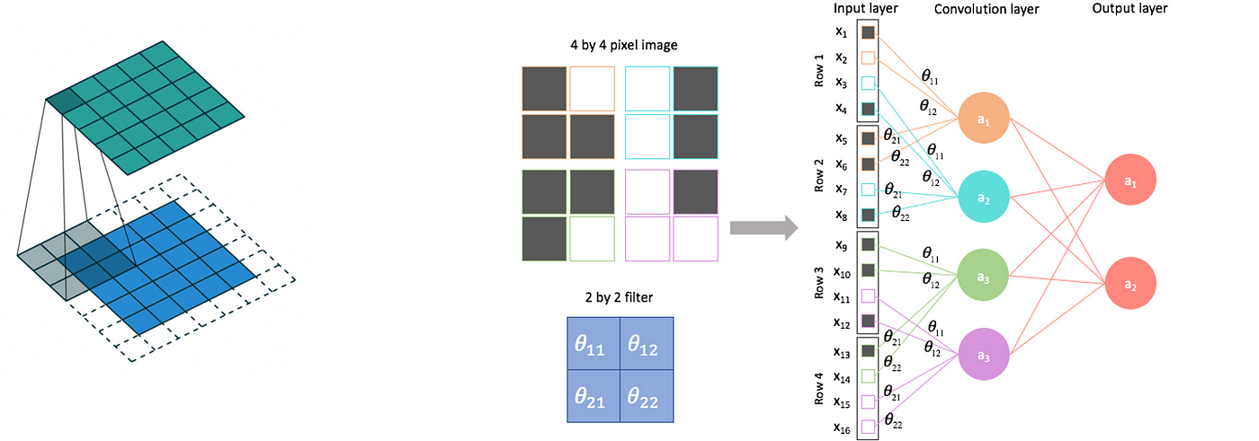
In short, a CNN can learn the above-mentioned local patterns by applying a convolution with shared weights: each node in a convolutional layer is the dot product between a window of adjacent nodes from the previous layer (pixels, in the case of a picture) and a matrix of weights.

Indeed, performing this product for all same-sized windows in the original layer amounts to applying a convolution operation: the convolving matrix, which is the same throughout the operation, is made of learnable network parameters which are thus shared between the nodes.

This way, translation invariance is enforced: the network learns to associate local patterns to the desired output, no matter the position of the pattern inside the tensor.

See here [11] for an excellent and more extensive explanation.

In a CNN, parameters are shared throughout the layer by sliding a window across it [11].

But can we successfully apply a CNN in a Time Series setting?

Well, surely the two necessary conditions mentioned at the beginning must hold:

a Time Series is naturally an ordered 1D array, and
usually points that are close in time form interesting patterns (trends, peaks, oscillations).

By sliding its convolutional array along the time axis, a CNN is often able to pick up repeating patterns in a series just like it can detect objects in a picture.

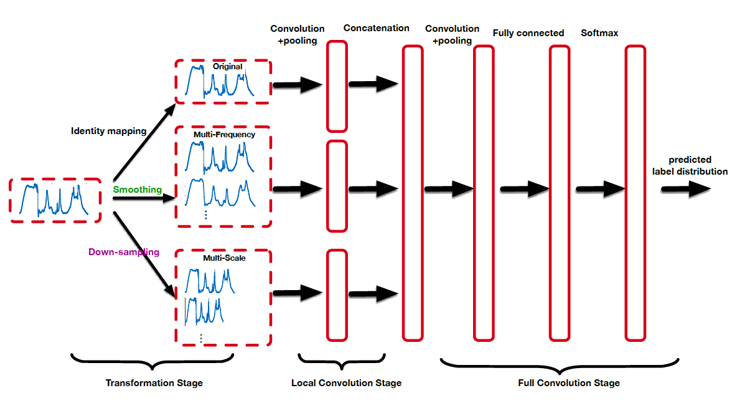
Moreover, we can trick a CNN into learning different structures by modifying its input series through well-known Time Series manipulation techniques.

For example, by sub-sampling a series we can make a convolutional layer detect patterns at different time scales; by applying transformations in the frequency domain we can make it learn smooth, de-noised patterns [12].

A convolutional network acting on transformed Time Series [12].

Recurrent Neural Networks

If CNNs found their sweet spot in Computer Vision applications, where images and videos are the most common data formats, Recurrent Neural Networks seem particularly suitable for Time Series applications.

Nonetheless, the most striking successes of RNNs arguably come from the field of Natural Language Processing, in tasks such as machine translation or speech recognition [17].

Indeed, while CNNs look for local structures inside multi-dimensional ordered data, RNNs focus on a single dimension and look for patterns of longer duration.

The ability to detect patterns that span across great lengths is particularly useful when dealing with certain types of Time Series, namely those that present low-frequency cycles and seasonalities or those having long-range auto-correlations.

A basic RNN layer acting on ordered 1D input data has a one-to-one association between those data points and the nodes of the layer; on top of this, intra-layer connections form a chain that follows the ordering of the input data.

The training process consists of splitting the sequential data into sliding, overlapping chunks (of the same length as the number of hidden states): they are fed sequentially, linked by the recurrent intra-layer connections that propagate through them.

We often denote layer nodes as latent or hidden states h; they encode meaningful information from their correspondent input data point, mediating it with the recursive signal from previous hidden states.

A basic RNN, folded (left) and unfolded (right) [13].

For Time Series forecasting purposes, the output nodes of a recurrent layer can be trained to learn an n-step-ahead prediction, for any choice of n, so that the ordered output represents a full forecast path; more often than not, though, an RNN is just a module in a more complex architecture.

In any case, the idea is to process and retain information about the past so that at any point during the training process the algorithm can access said information and use it.

As in CNNs, this is a form of weight sharing, since all chunks of the Time Series enter the same architecture; for the same reason, translation invariance assures that independently of when a certain pattern happened, the model will still be able to associate it to the observed output value.

In a plain RNN, hidden states are linked to input nodes and each other using classic activation functions and linear scalar products; a number of different more complex “flavours”, such as LSTMs and GRUs, have emerged in response to a few known limitations such as vanishing gradients [18][19].

In short, the vanishing gradient effect occurs during backpropagation, when composing small derivatives with the product rule in a long computation chain can result in infinitesimal updates in some nodes’ parameters, effectively halting the training algorithm [20].

Different RNN “flavours”: LSTM (left), and GRU (right) [14].

Attention Mechanisms

Attention Mechanisms were born in the context of NLP for the task of neural machine translation, where the idea of a single global model capable of translating any sentence from a given language required a more complex technique than those available at the time [22].

AMs are often found in Encoder-Decoder architectures, where they allow to capture mostly relevant information.

Example of actual use of an Attention Mechanism in an Encoder-Decoder architecture [15].

The general idea of an attention mechanism, indeed, is that treating all bits of a temporal data sequence as if they’re all equally important can be wasteful if not misleading for a model.

Some words can be fundamental for understanding the tone and context of a sentence: they need to be considered in conjunction with most other words in the same sentence.

In practical terms the model needs to stay alert, being ready to pay more attention to these words and to use them to influence its translation of others in the same sentence.

In Time Series applications, a similar argument can be made about moments in time that are critical and influential for future development of the series: structural trend changes, unexpected spikes (outliers), unusually long low-valued periods… are just some of the patterns that can be useful to detect in some contexts.

Practical application of a multi-head attention mechanism in Google’s TFT, detecting trend changes in a volatility series [10].

That’s basically what an AM does: it takes any given piece of input data (sometimes called query) and considers all possible input-output pairs (called keys and values respectively) conditionally on the presence of the query itself.

Attention Mechanism simplified in the QKV notation [15].

In the process, the model computes attention scores that signify the importance of the query as context for each key.

Note that the scoring function can be fixed (e.g. computing the distance between query and key in the sequence), or, more interestingly, parameterized in order to be learnable.

Attention scores are usually normalized into weights and used for a weighted average of values, which can be used as the output of the mechanism.

Possible design of an Attention Mechanism [15].

Residual Networks

Residual Networks are accessories to existing modules, providing what is called a skip connection: the input gets transported in parallel with the computation that happens to it in the block, and the two versions are then combined at the output (usually with an addition or a subtraction, with distinct effects).

In the case of an addition, for example, the introduction of a skip connection effectively makes it such that the skipped block switches from learning some original transformation f(x) to its residual, f(x)-x.

Essential structure of a residual network, where the dashed block is bypassed by a residual connection [15].

They were first introduced by applying them to CNNs [21], but nowadays they are basically everywhere since they provide clear advantages without adding too much computation or complexity.

From the look of them, RNs are a very simple concept; it is maybe not obvious what it achieves, though, so let’s now break down their strengths.

Facilitating information spread: as mentioned before, long chains of computation can suffer from vanishing gradients; a residual connection provides an additional term to the gradient that does not contain the chain product of derivatives given by the skipped block.
Avoiding accuracy saturation: it has been shown [21] that adding residual blocks helps mitigate this effect, which consists in blocking the usual improvements that come from adding more layers and sometimes can even cause deterioration instead (“degradation”).
Providing on/off switches: the fact that the skipped block learns the residual f(x)-x opens a new possibility for the model, namely to set all parameters of the block such that f(x)=0 and the combined output equals x. This is of course an identity, meaning that the combined block is effectively turned off.
Decomposing an input: another effect of learning residuals is that if you cleverly assemble residual blocks in series (“cascading” blocks), then the n-th block can be made to learn the result of removing the previous n-1 blocks from the input. In other words, each block is learning a little piece of the desired outcome, which can be recovered by adding together the pieces at the end. Moreover, we can tailor each cascading block to learn different pieces, so that we effectively achieve known Time Series decompositions, such as the STR or a Fourier transform [9].

Residual network assigning cascading blocks to different additive components of a Time Series in N-BEATS [9].

Hopefully, it is clear at this point that Deep Learning is on a successful path as far as Time Series forecasting goes.

This path represents a history of increasingly complex and tailored models, specializing in different sub-classes of Time Series, and it is only being populated by Neural Networks since recently; classical statistical models pre-date them, but still showed a tendency to get more and more handcrafted for specific predictive tasks.

In the future, and this consideration surely applies to other fields of Statistical Learning (especially Machine Learning), it is imperative for the somewhat artisanal approach commonly used today to make space for a mathematical framework that can systematically link the features of a prediction problem to the best possible architectures for solving it.

Building blocks for state-of-the-art models