
Time Series Classification for Fatigue Detection in Runners — A Tutorial
Time Series Classification for Fatigue Detection in Runners — A Tutorial
A step-by-step walkthrough of inter-participant and intra-participant classification performed on wearable sensor data of runners
Running data collected using wearable sensors can provide insights about a runner’s performance and overall technique. The data that comes from these sensors are usually time series by nature. This tutorial runs through a fatigue detection task where time series classification methods are used on a running dataset. In this tutorial, the time series data is used in its raw format rather than extracting features from the time series. This leads to an extra dimension in the data and hence traditional machine learning algorithms which use the data in a traditional vector format do not work well. Hence specific time series algorithms need to be used.
The data contains motion capture data from runners under normal and fatigued conditions. The data was collected using Inertial Measurement Units (IMU) at University College Dublin, Ireland. The data used in this tutorial can be found at https://zenodo.org/records/7997851 . The data presents a binary classification task where we try to predict between ‘Fatigued’ and ‘Non-Fatigued’. In this tutorial, we use the specialised Python packages, Scikit-learn; a toolkit for machine learning on python and sktime; a library specifically created for machine learning for time series.
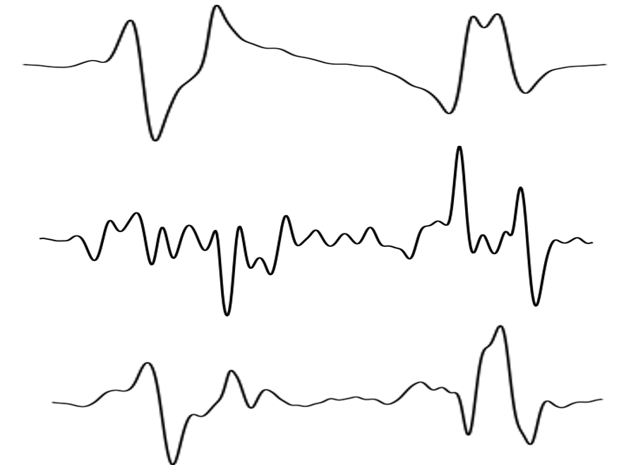
The dataset contains multiple channels of data. Here, we model the problem as a univariate problem for simplicity and hence only one channel of the data is used. We select the magnitude acceleration signal as it is the best performing signal [1, 2]. The magnitude signal is the square root of the squared sum of each of the directional components.
More detailed information about the data collection and processing can be found in the following papers, [1, 2].
To summarize, in this tutorial:
- A time series classification task is performed using a state-of-the-art time series classification technique on wearable sensor collected data.
- A comparison is made between the use of inter-participant models (globalised) and intra-participant models (personalised) for fatigue detection in runners.
Setup of the classification task
First, we need to load the data required for the analysis. For this evaluation, we use the data from “Accel_mag_all.csv”. We use pandas to load the data. Make sure you have downloaded this file from https://10.5281/zenodo.7997850 .
import pandas as pd

filename = "Accel_mag_all.csv"
data = pd.read_csv(filename, header = None)
A few functions from the sktime and sklearn packages are required so we load them below prior to beginning the analysis:
from sktime.transformations.panel.rocket import Rocket
from sklearn.pipeline import make_pipeline
from sklearn.preprocessing import StandardScaler
from sklearn.linear_model import RidgeClassifierCV, LogisticRegression, LogisticRegressionCV
from sklearn.model_selection import LeaveOneGroupOut
Next, we separate the labels and the participant number. Data will be represented by arrays from here.
import numpy as np

X = data.iloc[:,2:].values

y =  data[1].values
participant_no =  data[0].values
For this task, we are going to use the Rocket transform along with a Ridge Regression Classifier. Rocket is a state-of-the-art technique for time series classification [3]. Rocket works through the generation of random convolutional kernels which are convolved along the time series to produce a feature map. A simple linear classifier such as Ridge classifier is then used on this feature map. A pipeline can be created that first transforms the data using Rocket, standardizes the features, and finally uses the Ridge Classifier to do the classification.
rocket_pipeline_ridge = make_pipeline(
    Rocket(random_state=0),
    StandardScaler(),
    RidgeClassifierCV(alphas=np.logspace(-3, 3, 10))
)
Globalised Classification
In applications where we have data from multiple participants, using all the data together would mean that an individual’s data can appear in both training and test sets. To avoid this, a leave-one-subject-out (LOSO) analysis is generally performed where the model is trained on all but one participant and tested on the one left-out participant. This is repeated for every participant. This method would test the ability of the model to generalise between participants.
logo = LeaveOneGroupOut()

logo.get_n_splits(X, y, participant_no)

Rocket_score_glob = []
for i, (train_index, test_index) in enumerate(logo.split(X, y, participant_no)):
    rocket_pipeline_ridge.fit(X[train_index], y[train_index])

    Rocket_score = rocket_pipeline_ridge.score(X[test_index],y[test_index])
    Rocket_score_glob = np.append(Rocket_score_glob, Rocket_score)
Printing out a summary of results from above:
print("Global Model Results")
print(f"mean accuracy: {np.mean(Rocket_score_glob)}")
print(f"standard deviation: {np.std(Rocket_score_glob)}")
print(f"minimum accuracy: {np.min(Rocket_score_glob)}")
print(f"maximum accuracy: {np.max(Rocket_score_glob)}")
The output from the above code:
Global Model Results
mean accuracy: 0.5919805636306338
standard deviation: 0.10360659996594646
minimum accuracy: 0.4709480122324159
maximum accuracy: 0.8283582089552238
The accuracy from this LOSO analysis is notably low with some datasets yielding results that are as poor as random guessing. This suggests that the data from one participant may not generalise well to another participant. This is a commonly occurring issue when working with personal sensing data as the exercise technique and overall physiology are different from one individual to another. Furthermore, in this application, how one person compensates for fatigue may be different to how another person compensates for fatigue. Let’s see if we can improve the performance by personalising the models.
Personalised Classification
When building personalised models, the prediction is made based on the individual’s data. While splitting time series data into train and test sets, it should be done in a way where the data is not shuffled. To do this, we split each class into individual train and test sets to preserve the proportion of each class in the train and test sets while also preserving the time series nature of the data. The data from the first two-thirds of the run is used to train the model to predict on the last one-third of the run.
Rocket_score_pers = []
for i, (train_index, test_index) in enumerate(logo.split(X, y, participant_no)):

    #print(f"Participant: {participant_no[test_index][0]}")
    label = y[test_index]
    X_S = X[test_index]

    # Identify the indices for each class
    class_0_indices = np.where(label == 'NF')[0]
    class_1_indices = np.where(label == 'F')[0]

    # Split each class into train and test using indexing
    class_0_split_index = int(0.66 * len(class_0_indices))
    class_1_split_index = int(0.66 * len(class_1_indices))

    X_train = np.concatenate((X_S[class_0_indices[:class_0_split_index]], X_S[class_1_indices[:class_1_split_index]]), axis=0)
    y_train = np.concatenate((label[class_0_indices[:class_0_split_index]], label[class_1_indices[:class_1_split_index]]), axis=0)

    X_test = np.concatenate((X_S[class_0_indices[class_0_split_index:]],X_S[class_1_indices[class_1_split_index:]]), axis=0)
    y_test = np.concatenate((label[class_0_indices[class_0_split_index:]], label[class_1_indices[class_1_split_index:]]), axis=0)

    rocket_pipeline_ridge.fit(X_train, y_train)

    Rocket_score_pers = np.append(Rocket_score_pers, rocket_pipeline_ridge.score(X_test,y_test))
Printing out a summary of the results above as before:
print("Personalised Model Results")
print(f"mean accuracy: {np.mean(Rocket_score_pers)}")
print(f"standard deviation: {np.std(Rocket_score_pers)}")
print(f"minimum accuracy: {np.min(Rocket_score_pers)}")
print(f"maximum accuracy: {np.max(Rocket_score_pers)}")
Output from the above code:
Personalised Model Results
mean accuracy: 0.9517626092184379
standard deviation: 0.07750979452994386
minimum accuracy: 0.7037037037037037
maximum accuracy: 1.0
By personalising the models, a drastic improvement in the performance is seen. Hence, in this application, it is clear that there are difficulties in generalising from one person to another.
Conclusion
To perform a classification on the time series data from the wearable sensors, the state-of-the-art technique, Rocket was used. This analysis showed that in this domain personalising the models leads to better performing classification models.
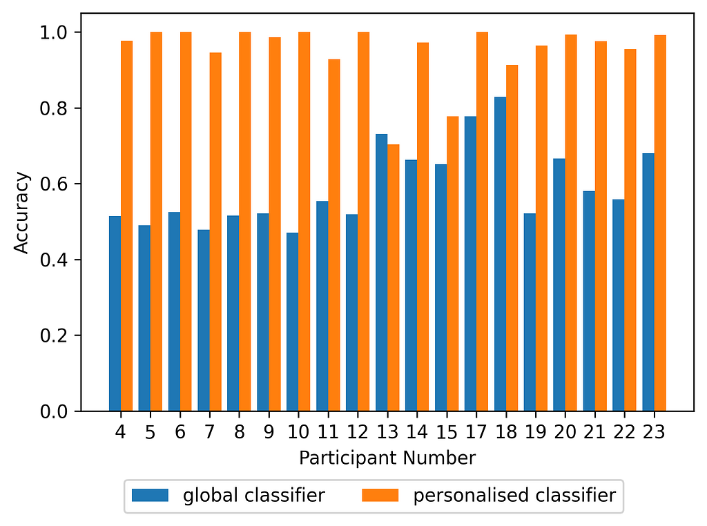
The above figure shows a big improvement in performance from using personalised models where for many participants, the performance almost doubles. The differences in physiology and running technique from one person to another are likely to contribute to this behaviour. From an user point of view, both global and personalised models would have benefits depending on the application. For example, in clinical settings where an individual users exercise technique needs to be monitored, a personalised model may be useful. However, collecting enough data from a single individual for accurate prediction can be difficult and hence for many applications, global models would be ideal.
The code presented in this tutorial can also be found on github: https://github.com/bahavathyk/TSC_for_Fatigue_Detection
References:
[1] B. Kathirgamanathan, T. Nguyen, G. Ifrim, B. Caulfield, P. Cunningham. Explaining Fatigue in Runners using Time Series Analysis on Wearable Sensor Data, XKDD 2023: 5th International Workshop on eXplainable Knowledge Discovery in Data Mining, ECML PKDD, 2023, http://xkdd2023.isti.cnr.it/papers/223.pdf
[2] B. Kathirgamanathan, B. Caulfield and P. Cunningham, “Towards Globalised Models for Exercise Classification using Inertial Measurement Units,” 2023 IEEE 19th International Conference on Body Sensor Networks (BSN), Boston, MA, USA, 2023, pp. 1–4, doi: 10.1109/BSN58485.2023.10331612.
[3] A. Dempster, F. Petitjean, and G. I.Webb. ROCKET: exceptionally fast and accurate time series classification using random convolutional kernels. Data Mining and Knowledge Discovery, 34(5):1454–1495, 2020.
Time Series Classification for Fatigue Detection in Runners — A Tutorial was originally published in Towards Data Science on Medium, where people are continuing the conversation by highlighting and responding to this story.
Time Series Classification for Fatigue Detection in Runners — A Tutorial
A step-by-step walkthrough of inter-participant and intra-participant classification performed on wearable sensor data of runners
Running data collected using wearable sensors can provide insights about a runner’s performance and overall technique. The data that comes from these sensors are usually time series by nature. This tutorial runs through a fatigue detection task where time series classification methods are used on a running dataset. In this tutorial, the time series data is used in its raw format rather than extracting features from the time series. This leads to an extra dimension in the data and hence traditional machine learning algorithms which use the data in a traditional vector format do not work well. Hence specific time series algorithms need to be used.
The data contains motion capture data from runners under normal and fatigued conditions. The data was collected using Inertial Measurement Units (IMU) at University College Dublin, Ireland. The data used in this tutorial can be found at https://zenodo.org/records/7997851 . The data presents a binary classification task where we try to predict between ‘Fatigued’ and ‘Non-Fatigued’. In this tutorial, we use the specialised Python packages, Scikit-learn; a toolkit for machine learning on python and sktime; a library specifically created for machine learning for time series.
The dataset contains multiple channels of data. Here, we model the problem as a univariate problem for simplicity and hence only one channel of the data is used. We select the magnitude acceleration signal as it is the best performing signal [1, 2]. The magnitude signal is the square root of the squared sum of each of the directional components.
More detailed information about the data collection and processing can be found in the following papers, [1, 2].
To summarize, in this tutorial:
- A time series classification task is performed using a state-of-the-art time series classification technique on wearable sensor collected data.
- A comparison is made between the use of inter-participant models (globalised) and intra-participant models (personalised) for fatigue detection in runners.
Setup of the classification task
First, we need to load the data required for the analysis. For this evaluation, we use the data from “Accel_mag_all.csv”. We use pandas to load the data. Make sure you have downloaded this file from https://10.5281/zenodo.7997850 .
import pandas as pd

filename = "Accel_mag_all.csv"
data = pd.read_csv(filename, header = None)
A few functions from the sktime and sklearn packages are required so we load them below prior to beginning the analysis:
from sktime.transformations.panel.rocket import Rocket
from sklearn.pipeline import make_pipeline
from sklearn.preprocessing import StandardScaler
from sklearn.linear_model import RidgeClassifierCV, LogisticRegression, LogisticRegressionCV
from sklearn.model_selection import LeaveOneGroupOut
Next, we separate the labels and the participant number. Data will be represented by arrays from here.
import numpy as np

X = data.iloc[:,2:].values

y =  data[1].values
participant_no =  data[0].values
For this task, we are going to use the Rocket transform along with a Ridge Regression Classifier. Rocket is a state-of-the-art technique for time series classification [3]. Rocket works through the generation of random convolutional kernels which are convolved along the time series to produce a feature map. A simple linear classifier such as Ridge classifier is then used on this feature map. A pipeline can be created that first transforms the data using Rocket, standardizes the features, and finally uses the Ridge Classifier to do the classification.
rocket_pipeline_ridge = make_pipeline(
    Rocket(random_state=0),
    StandardScaler(),
    RidgeClassifierCV(alphas=np.logspace(-3, 3, 10))
)
Globalised Classification
In applications where we have data from multiple participants, using all the data together would mean that an individual’s data can appear in both training and test sets. To avoid this, a leave-one-subject-out (LOSO) analysis is generally performed where the model is trained on all but one participant and tested on the one left-out participant. This is repeated for every participant. This method would test the ability of the model to generalise between participants.
logo = LeaveOneGroupOut()

logo.get_n_splits(X, y, participant_no)

Rocket_score_glob = []
for i, (train_index, test_index) in enumerate(logo.split(X, y, participant_no)):
    rocket_pipeline_ridge.fit(X[train_index], y[train_index])

    Rocket_score = rocket_pipeline_ridge.score(X[test_index],y[test_index])
    Rocket_score_glob = np.append(Rocket_score_glob, Rocket_score)
Printing out a summary of results from above:
print("Global Model Results")
print(f"mean accuracy: {np.mean(Rocket_score_glob)}")
print(f"standard deviation: {np.std(Rocket_score_glob)}")
print(f"minimum accuracy: {np.min(Rocket_score_glob)}")
print(f"maximum accuracy: {np.max(Rocket_score_glob)}")
The output from the above code:
Global Model Results
mean accuracy: 0.5919805636306338
standard deviation: 0.10360659996594646
minimum accuracy: 0.4709480122324159
maximum accuracy: 0.8283582089552238
The accuracy from this LOSO analysis is notably low with some datasets yielding results that are as poor as random guessing. This suggests that the data from one participant may not generalise well to another participant. This is a commonly occurring issue when working with personal sensing data as the exercise technique and overall physiology are different from one individual to another. Furthermore, in this application, how one person compensates for fatigue may be different to how another person compensates for fatigue. Let’s see if we can improve the performance by personalising the models.
Personalised Classification
When building personalised models, the prediction is made based on the individual’s data. While splitting time series data into train and test sets, it should be done in a way where the data is not shuffled. To do this, we split each class into individual train and test sets to preserve the proportion of each class in the train and test sets while also preserving the time series nature of the data. The data from the first two-thirds of the run is used to train the model to predict on the last one-third of the run.
Rocket_score_pers = []
for i, (train_index, test_index) in enumerate(logo.split(X, y, participant_no)):

    #print(f"Participant: {participant_no[test_index][0]}")
    label = y[test_index]
    X_S = X[test_index]

    # Identify the indices for each class
    class_0_indices = np.where(label == 'NF')[0]
    class_1_indices = np.where(label == 'F')[0]

    # Split each class into train and test using indexing
    class_0_split_index = int(0.66 * len(class_0_indices))
    class_1_split_index = int(0.66 * len(class_1_indices))

    X_train = np.concatenate((X_S[class_0_indices[:class_0_split_index]], X_S[class_1_indices[:class_1_split_index]]), axis=0)
    y_train = np.concatenate((label[class_0_indices[:class_0_split_index]], label[class_1_indices[:class_1_split_index]]), axis=0)

    X_test = np.concatenate((X_S[class_0_indices[class_0_split_index:]],X_S[class_1_indices[class_1_split_index:]]), axis=0)
    y_test = np.concatenate((label[class_0_indices[class_0_split_index:]], label[class_1_indices[class_1_split_index:]]), axis=0)

    rocket_pipeline_ridge.fit(X_train, y_train)

    Rocket_score_pers = np.append(Rocket_score_pers, rocket_pipeline_ridge.score(X_test,y_test))
Printing out a summary of the results above as before:
print("Personalised Model Results")
print(f"mean accuracy: {np.mean(Rocket_score_pers)}")
print(f"standard deviation: {np.std(Rocket_score_pers)}")
print(f"minimum accuracy: {np.min(Rocket_score_pers)}")
print(f"maximum accuracy: {np.max(Rocket_score_pers)}")
Output from the above code:
Personalised Model Results
mean accuracy: 0.9517626092184379
standard deviation: 0.07750979452994386
minimum accuracy: 0.7037037037037037
maximum accuracy: 1.0
By personalising the models, a drastic improvement in the performance is seen. Hence, in this application, it is clear that there are difficulties in generalising from one person to another.
Conclusion
To perform a classification on the time series data from the wearable sensors, the state-of-the-art technique, Rocket was used. This analysis showed that in this domain personalising the models leads to better performing classification models.
The above figure shows a big improvement in performance from using personalised models where for many participants, the performance almost doubles. The differences in physiology and running technique from one person to another are likely to contribute to this behaviour. From an user point of view, both global and personalised models would have benefits depending on the application. For example, in clinical settings where an individual users exercise technique needs to be monitored, a personalised model may be useful. However, collecting enough data from a single individual for accurate prediction can be difficult and hence for many applications, global models would be ideal.
The code presented in this tutorial can also be found on github: https://github.com/bahavathyk/TSC_for_Fatigue_Detection
References:
[1] B. Kathirgamanathan, T. Nguyen, G. Ifrim, B. Caulfield, P. Cunningham. Explaining Fatigue in Runners using Time Series Analysis on Wearable Sensor Data, XKDD 2023: 5th International Workshop on eXplainable Knowledge Discovery in Data Mining, ECML PKDD, 2023, http://xkdd2023.isti.cnr.it/papers/223.pdf
[2] B. Kathirgamanathan, B. Caulfield and P. Cunningham, “Towards Globalised Models for Exercise Classification using Inertial Measurement Units,” 2023 IEEE 19th International Conference on Body Sensor Networks (BSN), Boston, MA, USA, 2023, pp. 1–4, doi: 10.1109/BSN58485.2023.10331612.
[3] A. Dempster, F. Petitjean, and G. I.Webb. ROCKET: exceptionally fast and accurate time series classification using random convolutional kernels. Data Mining and Knowledge Discovery, 34(5):1454–1495, 2020.
Time Series Classification for Fatigue Detection in Runners — A Tutorial was originally published in Towards Data Science on Medium, where people are continuing the conversation by highlighting and responding to this story.
Denial of responsibility! Techno Blender is an automatic aggregator of the all world’s media. In each content, the hyperlink to the primary source is specified. All trademarks belong to their rightful owners, all materials to their authors. If you are the owner of the content and do not want us to publish your materials, please contact us by email – [email protected]. The content will be deleted within 24 hours.