
Tips and Tricks to Organize Jupyter Notebook Visualizations
Optimize your data science workflow by automating matplotlib output — with 1 line of code. Here’s how.
Naming things is hard. After a long enough day, we’ve all ended up with the highly-descriptive likes of “graph7(1)_FINAL(2).png” and “output.pdf" Look familiar?
We can do better — and quite easily, actually.
When we use data-oriented “seaborn-esque” plotting mechanisms, the ingredients for a descriptive filename are all there. A typical call looks like this,
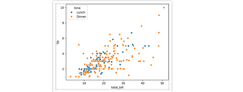
sns.scatterplot(data=tips, x="total_bill", y="tip", hue="time")
Right there we know we’ve got “total_bill” on the x axis, “time” color coded, etc. So what if we used the plotting function name and those semantic column keys to organize the output for us?
Here’s what that workflow looks like, using the teeplot tool.
import seaborn as sns; import teeplot as tp
tp.save = {".eps": True, ".pdf": True}  # set custom output behavior
tp.tee(sns.scatterplot,
   data=sns.load_data("tips"), x="total_bill", y="tip", hue="time")
teeplots/hue=time+viz=scatterplot+x=total-bill+y=tip+ext=.eps
teeplots/hue=time+viz=scatterplot+x=total-bill+y=tip+ext=.pdf
We’ve actually done three things in this example — 1) we rendered the plot in the notebook and 2) we’ve saved our visualization to file with a meaningful filename and 3) we’ve hooked our visualization into a framework where notebook outputs can be managed at a global level (in this case, enabling eps/pdf output).
This article will explain how to harness the teeplot Python package to get better organized and free up your mental workload to focus on more interesting things.
I am the primary author and maintainer of the project, which I have used in my own workflow for several years and found useful enough to package and share more widely with the community. teeplot is open source under the MIT license.
The teeplot Workflow
teeplot is designed to simplify work with data visualizations created with libraries like matplotlib, seaborn, and pandas. It acts as a wrapper around your plotting calls to handle output management for you.
Here’s how to use teeplot in 3 steps,
- Choose Your Plotting Function: Start by selecting your preferred plotting function, whether it’s from matplotlib, seaborn, pandas, etc. or one you wrote yourself.
- Add Your Plotting Arguments: Pass your plotting function as the first argument to tee, followed by the arguments you want to use for your visualization.
- Automatic Plotting and Saving: teeplot captures your plotting function and its arguments, executes the plot, and then takes care of wrangling the plot outputs for you.
That’s it!
Next, let’s look at 3 brief examples that demonstrate: a) basic use, b) custom post-processing, and c) custom plotting functions.
Example 1: Using a built-in pandas Plotter
In this example, we pass a DataFrame df’s member function df.plot.box as our plotter and two semantic keys: “age” and “gender.” teeplot takes care of the rest.
# adapted pandas.pydata.org/docs/reference/api/pandas.DataFrame.plot.box.html
import pandas as pd; from teeplot import teeplot as tp

age_list = [8, 10, 12, 14, 72, 74, 76, 78, 20, 25, 30, 35, 60, 85]
df = pd.DataFrame({"gender": list("MMMMMMMMFFFFFF"), "age": age_list})

tp.tee(df.plot.box,  # plotter...
    column="age", by="gender", figsize=(4, 3))  # ...forwa
teeplots/by=gender+column=age+viz=box+ext=.pdf
teeplots/by=gender+column=age+viz=box+ext=.png

Example 2: Matplotlib with Manual Tweaks
Like it or not, getting good results from matplotlib and its derivative libraries often requires some manual tweaks after the initial plotting call.
teeplot fully supports this pattern. Just pass the teeplot_callback kwarg, and teeplot will give you back a callable handle in addition to the output of the initial plotting call. After you’ve finished adjusting your plot, just invoke the handle to save and display as usual.
# adapted from https://matplotlib.org/stable/tutorials/pyplot.html
from matplotlib import pyplot as plt
import numpy as np; from teeplot import teeplot as tp

# tee output format can be configured globally (or per call to tp.tee)
tp.save = {".eps": True}  # make calls output to .eps only

# set up example data
df = {'weight': np.arange(50), 'profit': np.random.randint(0, 50, 50),
        'carbon': np.random.randn(50)}
df['price'], = df['weight'] + 10 * np.random.randn(50)
df['carbon'] = np.abs(df['carbon']) * 100

# ----- begin plotting -----
saveit, __ = tp.tee(  # --- "saveit" is callback to finalize output
    plt.scatter,  # plotter...
    data=df,  # then plotting kwargs
    x='weight', y='price', c='profit', s='carbon',
    teeplot_callback=True)  # defer plotting to callback

# tweak visualization as you usually would...
plt.xlabel('entry a')
plt.ylabel('entry b')
plt.gcf().set_size_inches(5, 3)
saveit()  # dispatch output callback
teeplots/c=profit+s=carbon+viz=scatter+x=weight+y=price+ext=.eps

Note the __ value unpacked from the tp.tee call above. This is because plt.scatter’s return value is a line collection that’s not useful for our tweaks.
Example 3: Custom Plotter
Custom plotters work just like external library plotters — teeplot can infer your plotting function’s name for the viz= output key.
from matplotlib import pyplot as plt; import seaborn as sns
from teeplot import teeplot as tp

def cuteplot(subject, descriptor, amount):  # custom plotter
    sns.dogplot()
    plt.gca().text(10, 400,
        f"{subject} \n is a {descriptor} dog" + "!" * amount,
        color="white", size=40)

tp.tee(cuteplot,  # plotter
    amount=4, subject="who", descriptor="good",  # plotting args
    teeplot_outinclude="amount")  # override to use numeric kwarg in filename
teeplots/amount=4+descriptor=good+subject=who+viz=cuteplot+ext=.png
teeplots/amount=4+descriptor=good+subject=who+viz=cuteplot+ext=.pdf

Shout-out sns.dogplot… always a howl!
Further Information

And that’s all there is to it!
I’ve been using this tool regularly for the last two years, and recently decided to take the time to package it up and share. Hope it can be an asset to the community.
The teeplot library has a few additional advanced features beyond what was covered here, like configurability via environment variables (useful in CI!). You can read more in the project’s usage guide and API listing. The project is open source on GitHub at mmore500/teeplot— consider leaving a ⭐️!
teeplot can be installed as python3 -m pip install teeplot
Authorship
This tutorial is contributed by me, Matthew Andres Moreno.

I currently serve as a postdoctoral scholar at the University of Michigan, where my work is supported by the Eric and Wendy Schmidt AI in Science Postdoctoral Fellowship, a Schmidt Futures program.
My appointment is split between the university’s Ecology and Evolutionary Biology Department, the Center for the Study of Complexity, and the Michigan Institute for Data Science.
Find me on Twitter as @MorenoMatthewA and on GitHub as @mmore500.
Disclaimer: I am the teeplot library author.
Citations
J. D. Hunter, “Matplotlib: A 2D Graphics Environment”, Computing in Science & Engineering, vol. 9, no. 3, pp. 90–95, 2007. https://doi.org/10.1109/MCSE.2007.55
Data structures for statistical computing in python, McKinney, Proceedings of the 9th Python in Science Conference, Volume 445, 2010. https://doi.org/ 10.25080/Majora-92bf1922–00a
Matthew Andres Moreno. (2023). mmore500/teeplot. Zenodo. https://doi.org/10.5281/zenodo.10440670
Waskom, M. L., (2021). seaborn: statistical data visualization. Journal of Open Source Software, 6(60), 3021, https://doi.org/10.21105/joss.03021.
Appendix
To install dependencies for examples in this article,
python3 -m pip install \
    matplotlib `# ==3.8.2`\
    numpy `# ==1.26.2` \
    teeplot `# ==1.0.1` \
    pandas `# ==2.1.3` \
    seaborn `# ==0.13.0`
Unless otherwise noted, all images are works of the author. “dogplot” image is via seaborn, find the a copy of the seaborn license here.
Tips and Tricks to Organize Jupyter Notebook Visualizations was originally published in Towards Data Science on Medium, where people are continuing the conversation by highlighting and responding to this story.
Optimize your data science workflow by automating matplotlib output — with 1 line of code. Here’s how.
Naming things is hard. After a long enough day, we’ve all ended up with the highly-descriptive likes of “graph7(1)_FINAL(2).png” and “output.pdf" Look familiar?
We can do better — and quite easily, actually.
When we use data-oriented “seaborn-esque” plotting mechanisms, the ingredients for a descriptive filename are all there. A typical call looks like this,
sns.scatterplot(data=tips, x="total_bill", y="tip", hue="time")
Right there we know we’ve got “total_bill” on the x axis, “time” color coded, etc. So what if we used the plotting function name and those semantic column keys to organize the output for us?
Here’s what that workflow looks like, using the teeplot tool.
import seaborn as sns; import teeplot as tp
tp.save = {".eps": True, ".pdf": True}  # set custom output behavior
tp.tee(sns.scatterplot,
   data=sns.load_data("tips"), x="total_bill", y="tip", hue="time")
teeplots/hue=time+viz=scatterplot+x=total-bill+y=tip+ext=.eps
teeplots/hue=time+viz=scatterplot+x=total-bill+y=tip+ext=.pdf
We’ve actually done three things in this example — 1) we rendered the plot in the notebook and 2) we’ve saved our visualization to file with a meaningful filename and 3) we’ve hooked our visualization into a framework where notebook outputs can be managed at a global level (in this case, enabling eps/pdf output).
This article will explain how to harness the teeplot Python package to get better organized and free up your mental workload to focus on more interesting things.
I am the primary author and maintainer of the project, which I have used in my own workflow for several years and found useful enough to package and share more widely with the community. teeplot is open source under the MIT license.
The teeplot Workflow
teeplot is designed to simplify work with data visualizations created with libraries like matplotlib, seaborn, and pandas. It acts as a wrapper around your plotting calls to handle output management for you.
Here’s how to use teeplot in 3 steps,
- Choose Your Plotting Function: Start by selecting your preferred plotting function, whether it’s from matplotlib, seaborn, pandas, etc. or one you wrote yourself.
- Add Your Plotting Arguments: Pass your plotting function as the first argument to tee, followed by the arguments you want to use for your visualization.
- Automatic Plotting and Saving: teeplot captures your plotting function and its arguments, executes the plot, and then takes care of wrangling the plot outputs for you.
That’s it!
Next, let’s look at 3 brief examples that demonstrate: a) basic use, b) custom post-processing, and c) custom plotting functions.
Example 1: Using a built-in pandas Plotter
In this example, we pass a DataFrame df’s member function df.plot.box as our plotter and two semantic keys: “age” and “gender.” teeplot takes care of the rest.
# adapted pandas.pydata.org/docs/reference/api/pandas.DataFrame.plot.box.html
import pandas as pd; from teeplot import teeplot as tp

age_list = [8, 10, 12, 14, 72, 74, 76, 78, 20, 25, 30, 35, 60, 85]
df = pd.DataFrame({"gender": list("MMMMMMMMFFFFFF"), "age": age_list})

tp.tee(df.plot.box,  # plotter...
    column="age", by="gender", figsize=(4, 3))  # ...forwa
teeplots/by=gender+column=age+viz=box+ext=.pdf
teeplots/by=gender+column=age+viz=box+ext=.png
Example 2: Matplotlib with Manual Tweaks
Like it or not, getting good results from matplotlib and its derivative libraries often requires some manual tweaks after the initial plotting call.
teeplot fully supports this pattern. Just pass the teeplot_callback kwarg, and teeplot will give you back a callable handle in addition to the output of the initial plotting call. After you’ve finished adjusting your plot, just invoke the handle to save and display as usual.
# adapted from https://matplotlib.org/stable/tutorials/pyplot.html
from matplotlib import pyplot as plt
import numpy as np; from teeplot import teeplot as tp

# tee output format can be configured globally (or per call to tp.tee)
tp.save = {".eps": True}  # make calls output to .eps only

# set up example data
df = {'weight': np.arange(50), 'profit': np.random.randint(0, 50, 50),
        'carbon': np.random.randn(50)}
df['price'], = df['weight'] + 10 * np.random.randn(50)
df['carbon'] = np.abs(df['carbon']) * 100

# ----- begin plotting -----
saveit, __ = tp.tee(  # --- "saveit" is callback to finalize output
    plt.scatter,  # plotter...
    data=df,  # then plotting kwargs
    x='weight', y='price', c='profit', s='carbon',
    teeplot_callback=True)  # defer plotting to callback

# tweak visualization as you usually would...
plt.xlabel('entry a')
plt.ylabel('entry b')
plt.gcf().set_size_inches(5, 3)
saveit()  # dispatch output callback
teeplots/c=profit+s=carbon+viz=scatter+x=weight+y=price+ext=.eps
Note the __ value unpacked from the tp.tee call above. This is because plt.scatter’s return value is a line collection that’s not useful for our tweaks.
Example 3: Custom Plotter
Custom plotters work just like external library plotters — teeplot can infer your plotting function’s name for the viz= output key.
from matplotlib import pyplot as plt; import seaborn as sns
from teeplot import teeplot as tp

def cuteplot(subject, descriptor, amount):  # custom plotter
    sns.dogplot()
    plt.gca().text(10, 400,
        f"{subject} \n is a {descriptor} dog" + "!" * amount,
        color="white", size=40)

tp.tee(cuteplot,  # plotter
    amount=4, subject="who", descriptor="good",  # plotting args
    teeplot_outinclude="amount")  # override to use numeric kwarg in filename
teeplots/amount=4+descriptor=good+subject=who+viz=cuteplot+ext=.png
teeplots/amount=4+descriptor=good+subject=who+viz=cuteplot+ext=.pdf
Shout-out sns.dogplot… always a howl!
Further Information
And that’s all there is to it!
I’ve been using this tool regularly for the last two years, and recently decided to take the time to package it up and share. Hope it can be an asset to the community.
The teeplot library has a few additional advanced features beyond what was covered here, like configurability via environment variables (useful in CI!). You can read more in the project’s usage guide and API listing. The project is open source on GitHub at mmore500/teeplot— consider leaving a ⭐️!
teeplot can be installed as python3 -m pip install teeplot
Authorship
This tutorial is contributed by me, Matthew Andres Moreno.
I currently serve as a postdoctoral scholar at the University of Michigan, where my work is supported by the Eric and Wendy Schmidt AI in Science Postdoctoral Fellowship, a Schmidt Futures program.
My appointment is split between the university’s Ecology and Evolutionary Biology Department, the Center for the Study of Complexity, and the Michigan Institute for Data Science.
Find me on Twitter as @MorenoMatthewA and on GitHub as @mmore500.
Disclaimer: I am the teeplot library author.
Citations
J. D. Hunter, “Matplotlib: A 2D Graphics Environment”, Computing in Science & Engineering, vol. 9, no. 3, pp. 90–95, 2007. https://doi.org/10.1109/MCSE.2007.55
Data structures for statistical computing in python, McKinney, Proceedings of the 9th Python in Science Conference, Volume 445, 2010. https://doi.org/ 10.25080/Majora-92bf1922–00a
Matthew Andres Moreno. (2023). mmore500/teeplot. Zenodo. https://doi.org/10.5281/zenodo.10440670
Waskom, M. L., (2021). seaborn: statistical data visualization. Journal of Open Source Software, 6(60), 3021, https://doi.org/10.21105/joss.03021.
Appendix
To install dependencies for examples in this article,
python3 -m pip install \
    matplotlib `# ==3.8.2`\
    numpy `# ==1.26.2` \
    teeplot `# ==1.0.1` \
    pandas `# ==2.1.3` \
    seaborn `# ==0.13.0`
Unless otherwise noted, all images are works of the author. “dogplot” image is via seaborn, find the a copy of the seaborn license here.
Tips and Tricks to Organize Jupyter Notebook Visualizations was originally published in Towards Data Science on Medium, where people are continuing the conversation by highlighting and responding to this story.
Denial of responsibility! Techno Blender is an automatic aggregator of the all world’s media. In each content, the hyperlink to the primary source is specified. All trademarks belong to their rightful owners, all materials to their authors. If you are the owner of the content and do not want us to publish your materials, please contact us by email – [email protected]. The content will be deleted within 24 hours.