
Total Interpretation of Basic Statistical R Commands | by Md Sohel Mahmood | Jul, 2022
Statistics in R Series
Introduction
R is a very powerful programming language for statistical analyses. There are several programming platforms for statistical analysis but R has gained real attraction among data scientists and data analysts because of its inherent capability to perform statistical tasks better than others and deliver the visualizations more aesthetically. In this article, I’m going to demonstrate the interpretation of very basic statistical commands executed in R. Anyone can perform the tasks on several other platforms but we need to understand the real idea behind its execution because these statistical concepts are timeless. The software, the program, the versions-everything can get updated but the concepts behind this statistical analysis will not change.
Data
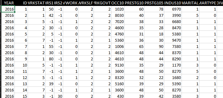
For demonstration, I will use the General Social Survey (GSS) data collected in 2016. The data were downloaded from the Association of Religion Data Archives and were collected by Tom W. Smith. This data set has responses collected from nearly 3,000 respondents and it has data related to several socio-economic features. For example, it has data related to marital status, education background, working hours, employment status, and many more. Let’s dive into this dataset I understand it a bit more.
The description of MARITAL and DEGREE encoded values are shown below since we will use these features in subsequent analyses.
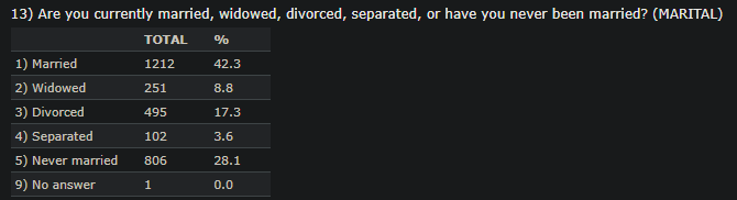
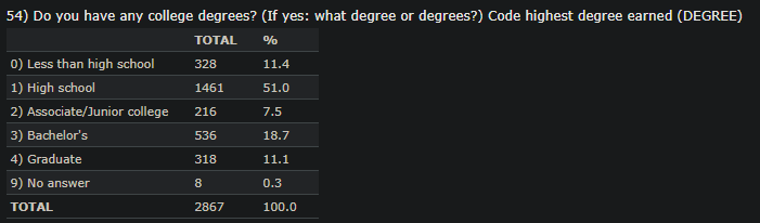
This data set comprises several features either quantitative or categorical. The categorical data are also encoded ordinally. For example, the education background has six different categories and each of these categories is assigned a number starting from 0. The gender is also categorical and only two values are assigned for this feature: “1” for males and “2” for females. There are also several quantitative data example age. To understand more about the assigned numbers, the reader needs to go to the given link and find out which number is associated with which categorical value. We will use this data and execute the following commands on both categorical and quantitative data and interpret the outputs.
The libraries are also shown here. I will use Rstudio. The goal is to understand the outputs from these commands, not emphasize the syntax.
Group_by
The group_by is one of the most basic and widely used commands for any sort of analysis. It groups the data based on the given feature variable. Once this group_by command is executed and stored in a variable, we can summarize that variable and display the desired statistics.
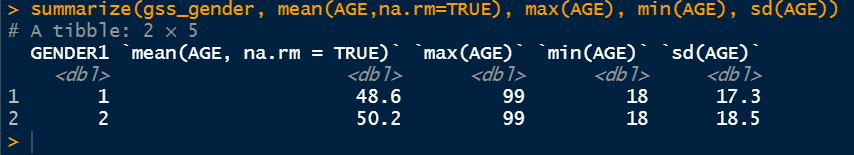
The above command shows the mean, the maximum, the minimum, and the standard deviation of age grouped by different genders which are very vital statistics for any dataset.
Group_by with descr
Other important statistics can be determined by combining descr command with group_by.
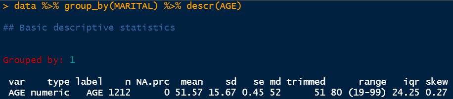
The above snap shows that the data is grouped by group 1 and the variable it is describing is AGE. The type of the variable is numeric and it has a total of 1212 data points the amount of null values is 0. It has a mean of 51.57 and a standard deviation of 15.67. Then we have a standard error which is denoted by se here. The standard error is the standard deviation divided by the total number of data points. In this case, it is 15.67/1212. Next, we have the median value which is 52. It says that the median age of the people belonging to group 1 is 52. Group 1 is the group for married people. Then we have the trimmed range which is showing here 51–80. It essentially eliminates a percentage of the lower and the upper data points but the real range is showing next which is 19–99. The IQR value is determined as 24.25 which is the difference between the third quartile and the first quartile (Q3-Q1). The IQR value is very handy to determine the upper limit and lower limit for box plots to eliminate the outliers. Finally, we have the skew value which is 0.27. This value indicates that the distribution is fairly normal. Any value above 1 is pretty much right-skewed and any value below -1 is considered left-skewed.
Statistics by selected features
We can also determine various statistics of different parameters using different libraries. One of those executions is shown below.
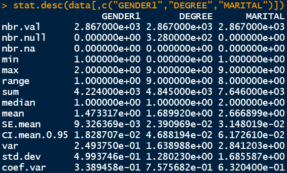
The output shows the total number of data points in the first row and the total number of null values in the second and the third row. Following that, we have the minimum and the maximum value as well as the range value. The sum, the median, the average, and the standard error are also shown in subsequent rows. We also have the value of 95% confidence interval mean data. Then, we also have the variance and the standard deviation values as well as the coefficient of variance. Variance is the square of standard deviation and coefficient of variance is the standard deviation divided by the mean. Standard deviation is the primary variable of interest to determine the spread of the desired parameter. However, coefficient of variance is another way to measure the spread in terms of the mean.
Table command
Table is a very powerful command to visualize the data split into two different groups. For example, in the following figure, the data is split into two groups: the first group is the marital status and the second group is the degree status.
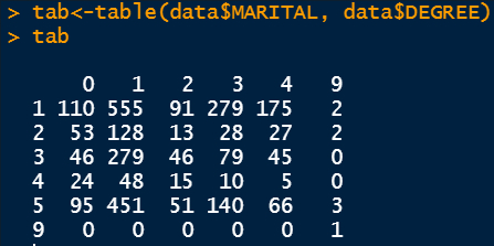
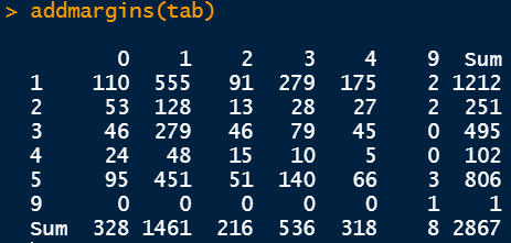
Since the categorical variables are encoded, we need to refer back to the description of the dataset to understand the underlying relation. For example 0 in the row refers to people having an education background less than high school and 1 in the column refers to people who are married. Therefore, 110 people have an education background less than high school and are married. There are different numbers as the education background changes.
Other miscellaneous commands
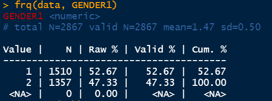
The frequency command denoted by frq determines important statistics of the selected feature. It shows the percentage values additionally as well as the cumulative percentages.
The summary command shows the Chi-Square test output if multiple factors are selected. We can feed the previously determined tab variable.
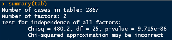
I would like to clarify these numbers from Chi-Square test. First of all, the tab variable holds the table data from marital status and education background status. What the Chi-Square test is doing is, it is checking the independence of one variable from another variable. Here, the Chi-Square test is checking if there is any dependency of the education background represented by DEGREE is somehow related to the marital status represented by MARITAL.
It does the calculation of p-value from the hypothesis test. The null hypothesis here states that the variables of interest (MARITAL and DEGREE) are not dependent on each other. The alternative hypothesis says that the variables are related and there may be some sort of correlation. In this case, the p-value is very small. The usual significance level is 5%. Since the p-value is less than 0.05, we can reject the null hypothesis and conclude that the education background is related to marital status.
The addmargins command provides the row and column summations.
Crosstable
Crosstable command is another very powerful command to visualize the table outputs and get more statistics.
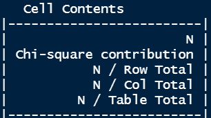
Apart from the amount (N), it also provides the Chi-Square contribution, the percentage towards the total of each row as well as each column, and the percentage of the total number.
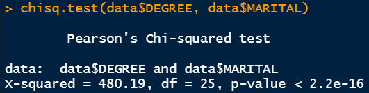
We can also determine the chi-square value and the corresponding p-value as shown below. It also provides the same statistics. The Chi-Square value is 480.19 and the degree of freedom is 25. In the output of the crosstable command, you can see the contribution of each segment towards this total Chi-Square value of 480.19. The degree of freedom value is calculated by multiplying (number of rows -1) and (number of columns -1).
Conclusion
We have covered the most basic interpretation of several vital R commands required for statistical analysis. These are required for both categorical and quantitative data analysis although the subsequent steps i.e. regression can be proceeded differently.
Thanks for reading.
Statistics in R Series

Introduction
R is a very powerful programming language for statistical analyses. There are several programming platforms for statistical analysis but R has gained real attraction among data scientists and data analysts because of its inherent capability to perform statistical tasks better than others and deliver the visualizations more aesthetically. In this article, I’m going to demonstrate the interpretation of very basic statistical commands executed in R. Anyone can perform the tasks on several other platforms but we need to understand the real idea behind its execution because these statistical concepts are timeless. The software, the program, the versions-everything can get updated but the concepts behind this statistical analysis will not change.
Data
For demonstration, I will use the General Social Survey (GSS) data collected in 2016. The data were downloaded from the Association of Religion Data Archives and were collected by Tom W. Smith. This data set has responses collected from nearly 3,000 respondents and it has data related to several socio-economic features. For example, it has data related to marital status, education background, working hours, employment status, and many more. Let’s dive into this dataset I understand it a bit more.
The description of MARITAL and DEGREE encoded values are shown below since we will use these features in subsequent analyses.
This data set comprises several features either quantitative or categorical. The categorical data are also encoded ordinally. For example, the education background has six different categories and each of these categories is assigned a number starting from 0. The gender is also categorical and only two values are assigned for this feature: “1” for males and “2” for females. There are also several quantitative data example age. To understand more about the assigned numbers, the reader needs to go to the given link and find out which number is associated with which categorical value. We will use this data and execute the following commands on both categorical and quantitative data and interpret the outputs.
The libraries are also shown here. I will use Rstudio. The goal is to understand the outputs from these commands, not emphasize the syntax.
Group_by
The group_by is one of the most basic and widely used commands for any sort of analysis. It groups the data based on the given feature variable. Once this group_by command is executed and stored in a variable, we can summarize that variable and display the desired statistics.
The above command shows the mean, the maximum, the minimum, and the standard deviation of age grouped by different genders which are very vital statistics for any dataset.
Group_by with descr
Other important statistics can be determined by combining descr command with group_by.
The above snap shows that the data is grouped by group 1 and the variable it is describing is AGE. The type of the variable is numeric and it has a total of 1212 data points the amount of null values is 0. It has a mean of 51.57 and a standard deviation of 15.67. Then we have a standard error which is denoted by se here. The standard error is the standard deviation divided by the total number of data points. In this case, it is 15.67/1212. Next, we have the median value which is 52. It says that the median age of the people belonging to group 1 is 52. Group 1 is the group for married people. Then we have the trimmed range which is showing here 51–80. It essentially eliminates a percentage of the lower and the upper data points but the real range is showing next which is 19–99. The IQR value is determined as 24.25 which is the difference between the third quartile and the first quartile (Q3-Q1). The IQR value is very handy to determine the upper limit and lower limit for box plots to eliminate the outliers. Finally, we have the skew value which is 0.27. This value indicates that the distribution is fairly normal. Any value above 1 is pretty much right-skewed and any value below -1 is considered left-skewed.
Statistics by selected features
We can also determine various statistics of different parameters using different libraries. One of those executions is shown below.
The output shows the total number of data points in the first row and the total number of null values in the second and the third row. Following that, we have the minimum and the maximum value as well as the range value. The sum, the median, the average, and the standard error are also shown in subsequent rows. We also have the value of 95% confidence interval mean data. Then, we also have the variance and the standard deviation values as well as the coefficient of variance. Variance is the square of standard deviation and coefficient of variance is the standard deviation divided by the mean. Standard deviation is the primary variable of interest to determine the spread of the desired parameter. However, coefficient of variance is another way to measure the spread in terms of the mean.
Table command
Table is a very powerful command to visualize the data split into two different groups. For example, in the following figure, the data is split into two groups: the first group is the marital status and the second group is the degree status.
Since the categorical variables are encoded, we need to refer back to the description of the dataset to understand the underlying relation. For example 0 in the row refers to people having an education background less than high school and 1 in the column refers to people who are married. Therefore, 110 people have an education background less than high school and are married. There are different numbers as the education background changes.
Other miscellaneous commands
The frequency command denoted by frq determines important statistics of the selected feature. It shows the percentage values additionally as well as the cumulative percentages.
The summary command shows the Chi-Square test output if multiple factors are selected. We can feed the previously determined tab variable.
I would like to clarify these numbers from Chi-Square test. First of all, the tab variable holds the table data from marital status and education background status. What the Chi-Square test is doing is, it is checking the independence of one variable from another variable. Here, the Chi-Square test is checking if there is any dependency of the education background represented by DEGREE is somehow related to the marital status represented by MARITAL.
It does the calculation of p-value from the hypothesis test. The null hypothesis here states that the variables of interest (MARITAL and DEGREE) are not dependent on each other. The alternative hypothesis says that the variables are related and there may be some sort of correlation. In this case, the p-value is very small. The usual significance level is 5%. Since the p-value is less than 0.05, we can reject the null hypothesis and conclude that the education background is related to marital status.
The addmargins command provides the row and column summations.
Crosstable
Crosstable command is another very powerful command to visualize the table outputs and get more statistics.
Apart from the amount (N), it also provides the Chi-Square contribution, the percentage towards the total of each row as well as each column, and the percentage of the total number.
We can also determine the chi-square value and the corresponding p-value as shown below. It also provides the same statistics. The Chi-Square value is 480.19 and the degree of freedom is 25. In the output of the crosstable command, you can see the contribution of each segment towards this total Chi-Square value of 480.19. The degree of freedom value is calculated by multiplying (number of rows -1) and (number of columns -1).
Conclusion
We have covered the most basic interpretation of several vital R commands required for statistical analysis. These are required for both categorical and quantitative data analysis although the subsequent steps i.e. regression can be proceeded differently.
Thanks for reading.
Denial of responsibility! Techno Blender is an automatic aggregator of the all world’s media. In each content, the hyperlink to the primary source is specified. All trademarks belong to their rightful owners, all materials to their authors. If you are the owner of the content and do not want us to publish your materials, please contact us by email – [email protected]. The content will be deleted within 24 hours.