
Training a Neural Network by Hand | by Brendan Artley | Jun, 2022
An introduction to the mathematics behind neural networks
Introduction
In this article, we will go through the mathematics behind training a simple neural network that solves a regression problem. We will use an input variable x to predict an output variable y. We will train two models by hand and then train a final model using Python.
Before starting, it would be good to know a little multivariate calculus, linear algebra, and linear regression to fully understand the mathematical processes explained in this article. If not, I would consider exploring Khan Academy as they have some great lessons on these topics.
Let’s start by defining a few data points to train the models on.
The first neural network will have an input layer with a single node and an output layer with a single node. The output layer will have a linear activation function. This is about as simple a neural network as you can get, but starting with this model makes the maths very intuitive. We will start by initializing the model with a weight of 0.5 and a bias of 0.
The easiest way initialize model parameters is to randomize the weights with values between 0 and 1 and initialize the biases values with 0. Other ways of setting starting parameters include He Initialization and Xavier initialization which aim to mitigate exploding/vanishing gradients and speed up convergence, but these are beyond the scope of this article.
Forward Pass
The first step is to pass our input variables through the model to gauge how well it performs. This is called a forward pass.
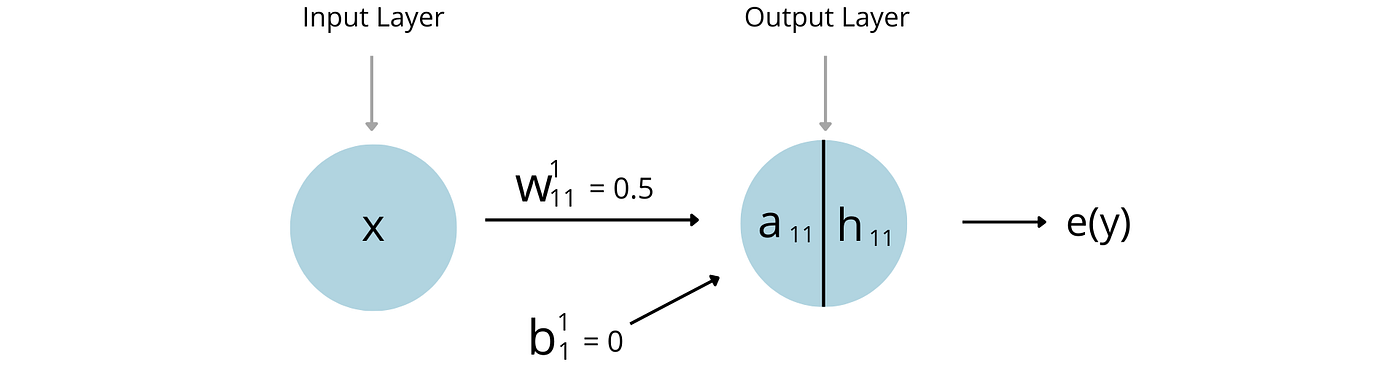
In the graphic above, a(x) is the linear combination of the inputs to that node, and h(x) is the activation function that transforms the a(x). As we are using a linear activation function the linear combinations of the input do not change.

The entire forward pass is denoted by the following function. This may look familiar as this is the equation of a straight line.

So, by plugging in each data point, we can solve the equation to get our initial model predictions.

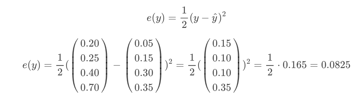
Then, we use an error function to determine how good our predictions are. In this case, we will be using 1/2 * MSE (mean squared error). The reason we multiply by a factor of 1/2 is that it reduces the number of coefficients in the chained partial derivatives that we compute during backpropagation. Don’t worry if this does not make sense, I will explain it later in the article. The formula and computation of 1/2 * MSE is shown below.
We can then visualize the initial predictions using matplotlib. In the following plot, the blue points are the true labels and the orange points are the predicted labels. The blue line shows how the neural network would classify other x values between 0–1. It is important to note that this line has a constant slope which is expected given the model equation is exactly that of a straight line.

Backpropagation
Looking at the graph above, you may be thinking that you can just pick a y-intercept and slope that makes better predictions. You would be right. In this section, we will use backpropagation to take a step in the right direction.
During backpropagation, we take the partial derivative of the error function with respect to each weight and bias in the model. The error function does not contain any weights or biases in its equation so we use the chain rule to do so. The result of doing this is a direction and magnitude in which each parameter should be tuned to minimize the error function. This concept is called gradient descent.
Chained Derivative for the Weight
Let’s start by computing the partial derivative of the error with respect to the weight value. I like to read the chained partial derivatives out loud as it makes the process easier to understand. For example in the following chained derivative, we are taking “the partial derivative of the error function with respect to the activation function h11, then we take the partial derivative of the activation function h11 with respect to the linear combination a11, and then we take the partial derivative of the linear combination a11 with respect to the weight w11.”

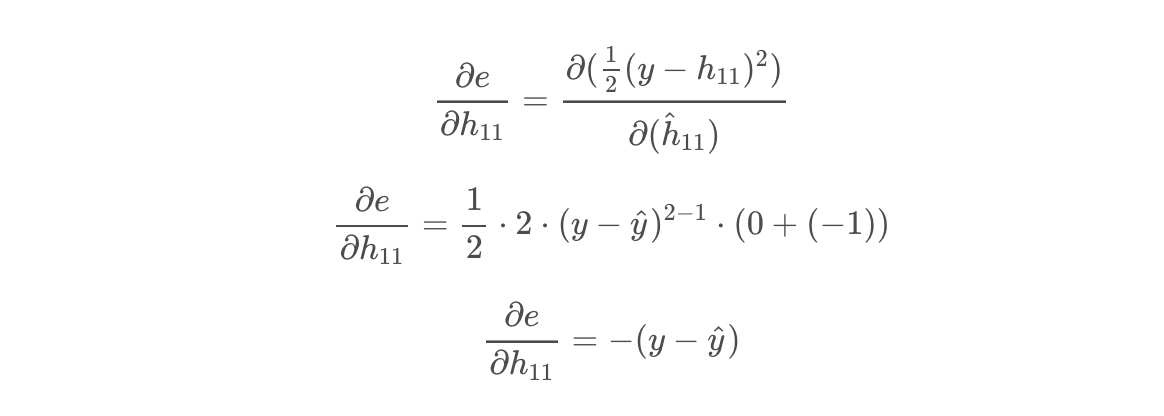
The first partial derivative we will compute is the partial derivative of the error function with respect to the activation function h11. This is where we see the the benefit of using 1/2 * MSE. By multiplying by a factor of 1/2 we are eliminating all coefficients (other than 1) in the resulting partial derivative.
Next, we take the partial derivative of the activation function h11 with respect to the linear combination a11. Since the activation is linear, this is essentially the partial derivative of a function with respect to itself, which is just 1.

Lastly, we take the partial derivative of the linear combination a11 with respect to the weight w11.

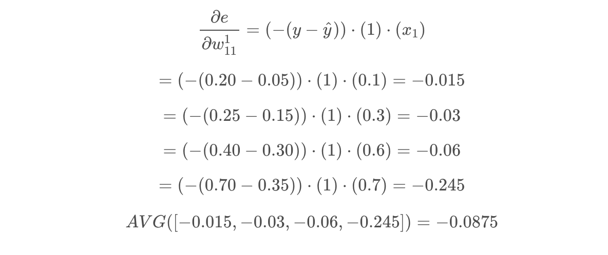
Putting it all together, we get the equation below. We can pass all the points through this equation and take the mean value to determine how we should change the w11 parameter to minimize the error function. This is called batch gradient descent. If we used a subset of the data points, this would be called mini-batch gradient descent.
Chained Derivative for the Bias
We are not done with partial derivatives just yet! We have to tune the bias value as well. This parameter is updated in a very similar way to the weight, with the exception of the final derivative in the chain. Thankfully we have already computed all but one of these derivatives in the section above.
The chained derivative for the bias term is shown below. Notice how similar it is to the chained derivative of the weight.

The only partial derivative we need to calculate is the partial derivative of the linear combination a11 with respect to the bias b11.

Putting it all together, we can solve the equation for each data point and take the average change that we should make to b11.

Updating the Weight
Now that we computed the partial derivatives for the weight we can update its value. The magnitude of the change made to the weight is dependent on a parameter called the learning rate. If the learning rate is too low, reaching the best model parameters will take a large number of epochs. If the learning rate is too high, we will constantly overshoot the best parameter combination. In this article, we will use a learning rate of 1. The learning rate is typically anywhere in the range of 0–1.
The formula for updating each weight is as follows. Note that the learning rate is denoted by alpha.

Updating the Bias
Then we can do the same with the bias. The formula for updating this is essentially the same as for the weights, with the magnitude of the change also being dependent on the learning rate.

Another Forward Pass
Now we have updated the weight and bias of the network, it should make better predictions.

Let’s perform another forward pass to confirm thats the case.

Then we evaluate how good the predictions are using 1/2 * MSE.

Wow! We were able to improve the error function from ~0.08 to ~0.02 in one epoch. In theory, we would keep updating the weight and bias until we stop improving on the error function. There are other things to consider in the real world such as overfitting the training data and using a validation set, but we will skip over this for now. Let’s visualize the predictions after 1 epoch.

I briefly mentioned before how this model is a simple linear regression model. This is because we are using a linear activation function, a single input, and single output node. If we increase the number of input nodes to increasing powers of x, we can build a linear regression model to any degree. This is pretty cool and is a great way transition to neural networks if you already understand linear regression models.
In this section we will fit a neural network with two input nodes (x and x²) and a single output node. Although still a simple network, this model will show how to create a linear regression model to the 2nd degree using neural networks.

Forward Pass
In this network the formula for the forward pass is slightly more complicated than the previous model.

Using our training data we can solve the equation for each data point. x1 is simply x, and x2 is x-squared.

Then as we did with the previous model, we evaluate the predictions with an error function (1/2 * MSE).

In the following plot, we can see that there is a slight convexity in the line (upwards curve) as we have added the second input parameter.

Backpropagation
Now we have made initial predictions, we can backpropagate to calculate how we should change the weights and bias. The three partial derivative chains that we need to calculate are as follows.

The first two partial derivatives of the three equations above are identical to those that we calculated with the previous model.

The final partial derivatives in each chain are as follows.
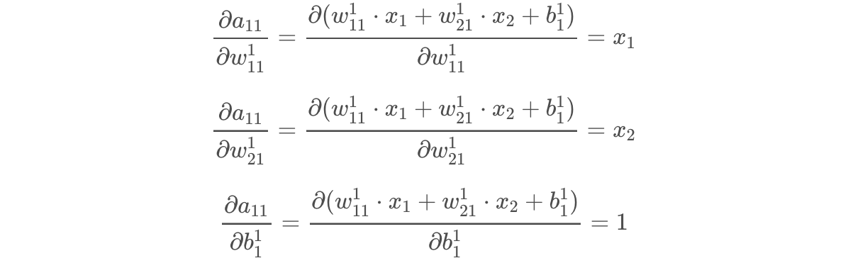
Then we can put each derivative chain together, solve for each data point, and take the average for each chain!


Next, we update the weights and the biases using the same formulas as before.

We will use a learning rate of 1 again. This triggers a large jump in the parameters and is good for visualizing a change in the model after 1 epoch. Typically you would set a lower learning rate and perform multiple epochs.

Another Forward Pass
Finally, we can perform another forward pass to see how much the model improved!

Awesome! We reduced the error function from ~0.06 to ~0.01. In the following cell we visualize this improvement. The more we train the model the closer we should get to fitting the data points exactly. The blue line is the updated model, and the grey line is the initial model.

3. Training a Neural Network with Code
Now that we have gone through all the mathematics, I want to show you how to train a model using Python. The computation we performed above can be done thousands of times a second by a computer. The following code block defines a neural network class for the model. I encourage you to look through the class functions and code comments to confirm this.
First, we instantiate the class and pass in our x and y values. Then we can then iteratively perform forward passes and backward propagation to update the model parameters. In the following example we are training the model for 3000 epochs, and logging the model predictions every 500 epochs.

As we can see the model continuously improves on its predictions, and after 2500 epochs we get a highly accurate model. As the model mirrors a linear regression model to the 2nd degree, it is limited to a convex function with scaling and transformations dependant on the model parameters. The training data points are not exactly a convex function and therefore we would need to increase the number of input nodes to fit the data perfectly.
I think the mathematics behind neural networks is pretty awesome. Hopefully working through a couple examples in this article with some sample data helped showcase this. Starting with a neural network that is a linear regression modes is good place to start, but the real predictive power of neural networks is unleashed when you add multiple layers and non-linear activation functions.
Code for this article can be found here.
Resources
- Training Neural Networks — Jeremy Jordan
- Activation Functions and Their Derivatives — Lakshmi Panneerselvam
- Backpropagation with RELU — StackExchange Discussion
- Weight Initialization Techniques — Saurabh Yadav
- Deep Learning Bias Backpropagation — Enes Zvornicanin
- Backpropagation Step-by-Step — Hani M. K.
An introduction to the mathematics behind neural networks

Introduction
In this article, we will go through the mathematics behind training a simple neural network that solves a regression problem. We will use an input variable x to predict an output variable y. We will train two models by hand and then train a final model using Python.
Before starting, it would be good to know a little multivariate calculus, linear algebra, and linear regression to fully understand the mathematical processes explained in this article. If not, I would consider exploring Khan Academy as they have some great lessons on these topics.
Let’s start by defining a few data points to train the models on.
The first neural network will have an input layer with a single node and an output layer with a single node. The output layer will have a linear activation function. This is about as simple a neural network as you can get, but starting with this model makes the maths very intuitive. We will start by initializing the model with a weight of 0.5 and a bias of 0.
The easiest way initialize model parameters is to randomize the weights with values between 0 and 1 and initialize the biases values with 0. Other ways of setting starting parameters include He Initialization and Xavier initialization which aim to mitigate exploding/vanishing gradients and speed up convergence, but these are beyond the scope of this article.
Forward Pass
The first step is to pass our input variables through the model to gauge how well it performs. This is called a forward pass.
In the graphic above, a(x) is the linear combination of the inputs to that node, and h(x) is the activation function that transforms the a(x). As we are using a linear activation function the linear combinations of the input do not change.
The entire forward pass is denoted by the following function. This may look familiar as this is the equation of a straight line.
So, by plugging in each data point, we can solve the equation to get our initial model predictions.
Then, we use an error function to determine how good our predictions are. In this case, we will be using 1/2 * MSE (mean squared error). The reason we multiply by a factor of 1/2 is that it reduces the number of coefficients in the chained partial derivatives that we compute during backpropagation. Don’t worry if this does not make sense, I will explain it later in the article. The formula and computation of 1/2 * MSE is shown below.
We can then visualize the initial predictions using matplotlib. In the following plot, the blue points are the true labels and the orange points are the predicted labels. The blue line shows how the neural network would classify other x values between 0–1. It is important to note that this line has a constant slope which is expected given the model equation is exactly that of a straight line.
Backpropagation
Looking at the graph above, you may be thinking that you can just pick a y-intercept and slope that makes better predictions. You would be right. In this section, we will use backpropagation to take a step in the right direction.
During backpropagation, we take the partial derivative of the error function with respect to each weight and bias in the model. The error function does not contain any weights or biases in its equation so we use the chain rule to do so. The result of doing this is a direction and magnitude in which each parameter should be tuned to minimize the error function. This concept is called gradient descent.
Chained Derivative for the Weight
Let’s start by computing the partial derivative of the error with respect to the weight value. I like to read the chained partial derivatives out loud as it makes the process easier to understand. For example in the following chained derivative, we are taking “the partial derivative of the error function with respect to the activation function h11, then we take the partial derivative of the activation function h11 with respect to the linear combination a11, and then we take the partial derivative of the linear combination a11 with respect to the weight w11.”
The first partial derivative we will compute is the partial derivative of the error function with respect to the activation function h11. This is where we see the the benefit of using 1/2 * MSE. By multiplying by a factor of 1/2 we are eliminating all coefficients (other than 1) in the resulting partial derivative.
Next, we take the partial derivative of the activation function h11 with respect to the linear combination a11. Since the activation is linear, this is essentially the partial derivative of a function with respect to itself, which is just 1.
Lastly, we take the partial derivative of the linear combination a11 with respect to the weight w11.
Putting it all together, we get the equation below. We can pass all the points through this equation and take the mean value to determine how we should change the w11 parameter to minimize the error function. This is called batch gradient descent. If we used a subset of the data points, this would be called mini-batch gradient descent.
Chained Derivative for the Bias
We are not done with partial derivatives just yet! We have to tune the bias value as well. This parameter is updated in a very similar way to the weight, with the exception of the final derivative in the chain. Thankfully we have already computed all but one of these derivatives in the section above.
The chained derivative for the bias term is shown below. Notice how similar it is to the chained derivative of the weight.
The only partial derivative we need to calculate is the partial derivative of the linear combination a11 with respect to the bias b11.
Putting it all together, we can solve the equation for each data point and take the average change that we should make to b11.
Updating the Weight
Now that we computed the partial derivatives for the weight we can update its value. The magnitude of the change made to the weight is dependent on a parameter called the learning rate. If the learning rate is too low, reaching the best model parameters will take a large number of epochs. If the learning rate is too high, we will constantly overshoot the best parameter combination. In this article, we will use a learning rate of 1. The learning rate is typically anywhere in the range of 0–1.
The formula for updating each weight is as follows. Note that the learning rate is denoted by alpha.
Updating the Bias
Then we can do the same with the bias. The formula for updating this is essentially the same as for the weights, with the magnitude of the change also being dependent on the learning rate.
Another Forward Pass
Now we have updated the weight and bias of the network, it should make better predictions.
Let’s perform another forward pass to confirm thats the case.
Then we evaluate how good the predictions are using 1/2 * MSE.
Wow! We were able to improve the error function from ~0.08 to ~0.02 in one epoch. In theory, we would keep updating the weight and bias until we stop improving on the error function. There are other things to consider in the real world such as overfitting the training data and using a validation set, but we will skip over this for now. Let’s visualize the predictions after 1 epoch.
I briefly mentioned before how this model is a simple linear regression model. This is because we are using a linear activation function, a single input, and single output node. If we increase the number of input nodes to increasing powers of x, we can build a linear regression model to any degree. This is pretty cool and is a great way transition to neural networks if you already understand linear regression models.
In this section we will fit a neural network with two input nodes (x and x²) and a single output node. Although still a simple network, this model will show how to create a linear regression model to the 2nd degree using neural networks.
Forward Pass
In this network the formula for the forward pass is slightly more complicated than the previous model.
Using our training data we can solve the equation for each data point. x1 is simply x, and x2 is x-squared.
Then as we did with the previous model, we evaluate the predictions with an error function (1/2 * MSE).
In the following plot, we can see that there is a slight convexity in the line (upwards curve) as we have added the second input parameter.
Backpropagation
Now we have made initial predictions, we can backpropagate to calculate how we should change the weights and bias. The three partial derivative chains that we need to calculate are as follows.
The first two partial derivatives of the three equations above are identical to those that we calculated with the previous model.
The final partial derivatives in each chain are as follows.
Then we can put each derivative chain together, solve for each data point, and take the average for each chain!
Next, we update the weights and the biases using the same formulas as before.
We will use a learning rate of 1 again. This triggers a large jump in the parameters and is good for visualizing a change in the model after 1 epoch. Typically you would set a lower learning rate and perform multiple epochs.
Another Forward Pass
Finally, we can perform another forward pass to see how much the model improved!
Awesome! We reduced the error function from ~0.06 to ~0.01. In the following cell we visualize this improvement. The more we train the model the closer we should get to fitting the data points exactly. The blue line is the updated model, and the grey line is the initial model.
3. Training a Neural Network with Code
Now that we have gone through all the mathematics, I want to show you how to train a model using Python. The computation we performed above can be done thousands of times a second by a computer. The following code block defines a neural network class for the model. I encourage you to look through the class functions and code comments to confirm this.
First, we instantiate the class and pass in our x and y values. Then we can then iteratively perform forward passes and backward propagation to update the model parameters. In the following example we are training the model for 3000 epochs, and logging the model predictions every 500 epochs.
As we can see the model continuously improves on its predictions, and after 2500 epochs we get a highly accurate model. As the model mirrors a linear regression model to the 2nd degree, it is limited to a convex function with scaling and transformations dependant on the model parameters. The training data points are not exactly a convex function and therefore we would need to increase the number of input nodes to fit the data perfectly.
I think the mathematics behind neural networks is pretty awesome. Hopefully working through a couple examples in this article with some sample data helped showcase this. Starting with a neural network that is a linear regression modes is good place to start, but the real predictive power of neural networks is unleashed when you add multiple layers and non-linear activation functions.
Code for this article can be found here.
Resources
- Training Neural Networks — Jeremy Jordan
- Activation Functions and Their Derivatives — Lakshmi Panneerselvam
- Backpropagation with RELU — StackExchange Discussion
- Weight Initialization Techniques — Saurabh Yadav
- Deep Learning Bias Backpropagation — Enes Zvornicanin
- Backpropagation Step-by-Step — Hani M. K.
Denial of responsibility! Techno Blender is an automatic aggregator of the all world’s media. In each content, the hyperlink to the primary source is specified. All trademarks belong to their rightful owners, all materials to their authors. If you are the owner of the content and do not want us to publish your materials, please contact us by email – [email protected]. The content will be deleted within 24 hours.