
Twitter Sentiment Analysis Using LSTM | by Bruno Caraffa
A detailed look at the power of LSTM applied to sentiment analysis
When you get in the driver’s seat of your car, are you able to just turn the engine on and drive away or do you need to think about how will you do it and each step of the process before leaving with the car? For most people, it’s the first option.
That’s also how recurrent neural networks (RNNs) work. You don’t need to think from the scratch about every basic task you will do on your day because we have a little thing called memory, and so do the recurrent neural networks. But how do they learn and store these memories?

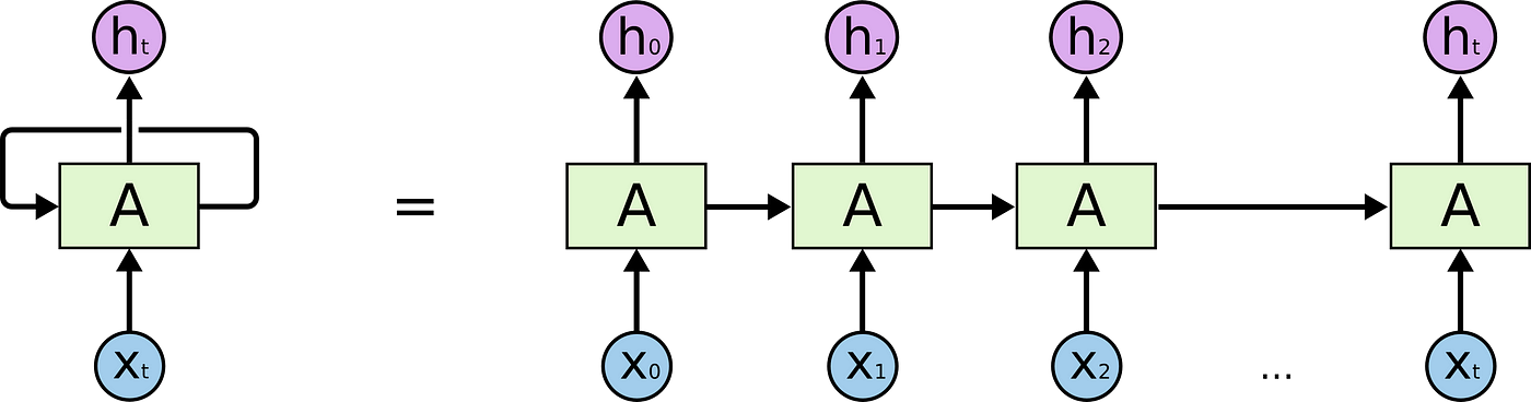
In the above diagram, a cell of a neural network receives some type of input Xt and outputs a value Ht. Then, the loop provides the information to the next cell, and so on. Therefore, the RNNs can be thought of as copies of the same network, each passing the information to the next. It’s easier to understand when we look at a complete chain, and it’s the loop shown in the image above unfolded:
RNNs have been applied with success to many kinds of natural language processing projects in the past few years. Those applications include speech recognition, language modeling, translation, and, of course, sentiment analysis that we will explore in this article. None of this would be possible without a special kind of RNN, and that is the LSTM (Long short-term memory). For many purposes, LSTMs work better than traditional recurrent networks, and here we will show how and why. But first, we need to talk about why can’t we just use the normal RNNs and what is the problem with it.
One of the exciting things about RNNs is that they can use past information in their predictions. Consider a model trying to predict the last word of a sentence based on the previous words. In the sentence: “The book is on the table” it’s a narrow range of options for the last word and “table” would be a great prediction with not much additional context needed for the prediction to be correct. In such cases that the distance between the relevant words to the prediction is small, the RNNs can predict well. However, what would happen if we needed more context for the word prediction?
Consider the sentence “I’ve been studying a lot these last few days and on the table, there is a book”. Recent information suggest that there is some object on the table, but if we want to narrow down to which object, we should go further back on the sentence. Then, if we look at the word “studying” in the first sentence, we would get the additional context needed for the prediction to be correct. As the sentence begins with “I’ve been studying” is much less likely that there is a football or a vodka bottle on the table rather than a pen or a book. And that is exactly why LSTM models are widely used nowadays, as they are particularly designed to have a long-term “memory” that is capable of understanding the overall context better than other neural networks affected by the long-term dependency problem.
The key to understanding how the LSTM work is the cell state. The cell state runs the entire chain with some minor linear interactions, and in those interactions, the LSTM can add or remove information with structures called gates. There are two gates: a sigmoid neural net layer and a pointwise multiplication operation.
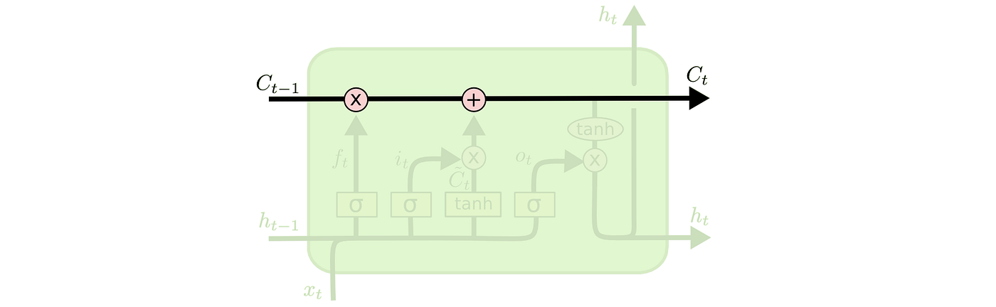
Gates are responsible for choosing which information will pass through. The sigmoid layer, for instance, applies a sigmoid function to the original vector and outputs a value between 0 and 1. And what does that mean? A value of zero would block all the information and a value of one would let all the information pass through the first gate and go on in the cell state flux.

As we’ve said, the first decision of the LSTM comes in the sigmoid layer gate, which we can also call the “forget” gate. The layer looks at two inputs: Xt, with the vectorized text, that we’re looking to predict the sentiment (with the help of a tokenizer, as can be seen on the image below), and Ht-1 with the previous information the model already had. Then, the sigmoid function is applied and it outputs a number between 0 and 1 for each cell state Ct-1.

We’ll do not go into details on the other LSTM layers in this article as the focus is on showing how to apply it for Twitter sentiment analysis, but the walkthrough of the algorithm is brilliantly explained in detail here. Now that we’ve talked plenty about the LSTM theory, let’s code and show how to use it to predict the sentiment of tweets.
Initially, we need to get a dataset with classified tweets to train and test our model. I’ve chosen the dataset of Kaggle’s Tweet Sentiment Extraction competition. This dataset is a collection of approximately 27.500 tweets.
So, let’s load our data:
import pandas as pddf_train = pd.read_csv('train.csv',sep=',')
df_train.text=df_train.text.astype(str)
df_val = pd.read_csv('test.csv',sep=',')
df_val.text=df_val.text.astype(str)

With the data already loaded, our next step is to merge the training and validation datasets to create a single dataset to which we can apply the pre-processing steps, especially the tokenizing process, which later we’ll explain in detail.
df = pd.concat([df_train.assign(ind="train"),df_val.assign(ind="validation")])
Now, the next step is to remove the neutral sentiments. It’s not a consensus, but some articles show that neutral word removal is a way to enhance the performance of a sentiment analysis model. It’s easier to interpret the results of binary classification and the models tend to perform better. Also, as we’re gonna work with arrays is necessary to convert the “positive” labels to 1 and the “negative” to 0.
df = df.loc[(df['sentiment'] == 'Positive') | (df['sentiment'] == 'Negative')]df.loc[df['sentiment'] == 'Positive','sentiment'] = 1 df.loc[df['sentiment'] == 'Negative','sentiment'] = 0
Now the fun begins! Let’s start manipulating the tweets and pre-processing them to prepare the input of our LSTM model. For this, we’ll need to load two libs: Spacy and RE (Regular Expressions). Spacy is an amazing natural language processing lib with some tools like pre-trained word vectors, lemmatization, stored stopwords, entity recognition, and others for more than 60 languages. All we must do is to install Spacy on our Python environment and download the language we want, in this article English. We’ll then download en_core_web_sm that is an English-trained pipeline, on its smaller version (the medium and large versions are also available). Then, we use the spacy function “load” to apply the pipeline we’ve just downloaded to the “nlp” object.
# pip install -U spacy
# python -m spacy download en_core_web_smimport spacy
nlp = spacy.load('en_core_web_sm')
import re
Now that the NLP libraries are loaded, we can start the text preprocessing. First, we should convert our text column to string and then we can remove the stopwords and apply the lemmatization with a single line of code using the methods “lemma_” and “is_stop” from the nlp-loaded pipeline we’ve just created above. Then, we must convert our strings to lowercase and use the regular expressions library so we can remove the whitespaces (\s) and the alphanumeric characters (\w), leaving only the words that matter to our model.
df["text"] = df["text"].astype(str)
df["text"] = df['text'].apply(lambda x: " ".join([y.lemma_ for y in nlp(x) if not y.is_stop]))
df['text'] = df['text'].apply(lambda x: x.lower())
df['text'] = df['text'].apply((lambda x: re.sub('[^\w\s]','',x)))
Now it’s time to vectorize our tweets, and we’ll do that using the Keras library preprocessing utilities. First, we must define the maximum number of words to keep based on the word frequency, we’ll set that to 3000 to have a solid variety of words in our vectors. When we fit the tokenizer onto the text is important that we do it on the full data (df), otherwise, if we fit the tokenizer only to the training tweets and then try to transform the validation dataset using the same tokenizer, we would probably get an error. There will be words that only show up on the validation dataset and are unknown to the tokenizer as it was fit using exclusively the train dataset words. Therefore, we’ll fit our tokenizer object to our full dataset.
from tensorflow.keras.preprocessing.text import Tokenizer
from tensorflow.keras.preprocessing.sequence import pad_sequencesmax_features = 3000
tokenizer = Tokenizer(num_words=max_features, split=' ')
tokenizer.fit_on_texts(df['text'].values)
Another problem with fitting the tokenizer only to the training dataset is the output’s shape. For instance, let’s imagine our train dataset has only one tweet with the example shown above “le chat est noir”. After the tokenization, we would get an array with shapes (1,4). Then, if we try predicting the sentiment of a tweet “I am happy”, an array with shapes (1,3), it wouldn’t be possible as the shapes of those arrays don’t match. In that case, we can fill the test array with a 0, using the numpy lib pad, to match the tokenizer’s original shape of (1,4). After doing that we would still have the not fitted words problem mentioned in the last paragraph, as none of the words “I”, “am” or “happy” are fit to the tokenizer and in the end our array would be [0,0,0,0]. The shape of the tokenizer can be set to a limit using the max_features parameter, but usually, it’s the same shape as the largest element, or in our case the tweet with the most words.
Now that the tokenizer has been fit to the full data frame we can split back to the train and validation datasets.
df_train, df_val = df[df["ind"].eq("train")], df[df["ind"].eq("validation")]
After splitting back df_train and df_val and fitting the tokenizer, it’s time to vectorize the tweets. That can be done using Keras’ texts_to_sequences and pad_sequences.
X_train = tokenizer.texts_to_sequences(df_train['text'].values)
X_train = pad_sequences(X_train)X_val = tokenizer.texts_to_sequences(df_val['text'].values)
X_val = pad_sequences(X_val)

After vectorizing the tweets it’s time to check if the shapes of our datasets match, otherwise we’ll need to adapt one of them.
[X_train.shape,X_val.shape]
The output we get is [(16.363, 20),(2.104, 18)], meaning that the X_train dataset has 16.363 rows (or tweets) and 20 features (or words) and the X_val dataset has 2.104 rows (or tweets) and 18 features (or words). Therefore, we’ll need to fill the X_val dataset with 0s to match the 20 features of X_train. But how can we do that to an array? Numpy, of course! Using the numpy lib pad, we can use X_train’s shape to subtract X_val’s shape to get the difference in features (or words) among the two arrays and fill X_val with a constant value of 0 to match the shapes.
import numpy as np
X_val = np.lib.pad(X_val, ((0,0),(X_train.shape[1] - X_val.shape[1],0)), 'constant', constant_values=(0))
X_val.shape

The output we get is (2.104,20), and finally, the training and validation arrays have the same features length (20) and can be used on our predictions. Now the last step in our preprocessing is to prepare our target values, so we’re gonna get the dummies out of those variables and turn them into arrays to use in our training and validation.
Y_train = np.array(pd.get_dummies((df_train['sentiment']).values))
Y_val = np.array(pd.get_dummies((df_val['sentiment']).values))
With the training and validation arrays all set, it’s time to build our LSTM model! But from where do we begin? Keras! One of the most loved libraries for deep learning and neural networks, it runs on top of the machine learning library TensorFlow. It allows us to build a model and using the sequential class on Keras, we can group a linear stack of layers into our model. Those are the same layers we mentioned in the LSTM explanation in the first part of this article.
from tensorflow.keras.models import Sequential
from tensorflow.keras.layers import Dense, Embedding, LSTM, SpatialDropout1D
Now the first step in building our LSTM network is creating an embedding layer. An embedding layer allows us to convert each word into a fixed-length vector and that is a better way to represent those words along with reduced dimensions. The max_features parameter is the size of the vocabulary that we’ve already set on the tokenization, the embed_dim parameter is the length of the vector we want for each word and input_length is the maximum length of a sequence, so in our case, we can use X_train.shape[1], which outputs 20. And that’s it, our embedding layer it’s done.
max_features = 3000
embed_dim = 128model = Sequential()
model.add(Embedding(max_features, embed_dim,input_length = X_train.shape[1]))
Moving on, after our embedding layer, it’s time to add a Spatial Dropout 1D layer to our model. The main purpose of the spatial dropout layer is to avoid overfitting and that is done by probabilistically removing the inputs of this layer (or the output of the embedding layer in the network we’re building). All in all, it has the effect of simulating many different networks (by dropping random elements, or in our case 30% of them — 0.3 parameter on the code) and in the end, the nodes of the network are more robust to the future inputs and tend to not overfit.
model.add(SpatialDropout1D(0.3))
Finally, it’s time to add our star layer, the one we’ve talked so much about, the one and only LSTM! The first parameter lstm_out that we’ve defined as 256 it’s the dimensionality of the output space, and we can choose an even larger number trying to improve our model, but that can lead to many problems like overfitting and a long training time. The dropout parameter is applied to the inputs and/or outputs of our model (the linear transformations), while the recurrent dropout is applied to the recurrent state, or cell state, of the model. In other words, the recurrent dropout affects the “memory” of the network. For this LSTM network, I’ve chosen to work with a larger dropout and recurrent dropout of 0.5 as we’ve got a small dataset and that is an important step to avoid overfitting.
lstm_out = 256model.add(LSTM(lstm_out, dropout=0.5, recurrent_dropout=0.5))
Now that our LSTM layer it’s done is time to prepare our activation function. We do that by adding a densely-connected layer to implement the activation function to our network and output the dimensionality we want for our final array. As we’ve seen before, in LSTM we need a sigmoid neural net layer and that is exactly why we’ve chosen the sigmoid activation. The sigmoid function outputs a value between 0 and 1 and it can either let no flow or complete flow of information throughout the gates.
Finally, we are ready to compile the model, which is configuring the model for training. We’ll select the categorical cross-entropy for our loss function, which is a widely used loss function to quantify deep learning model errors in classification problems. For our optimizer, we’ll go with the Adam optimizer, an implementation of the Adam algorithm, which is a robust extended version of the stochastic gradient descent and is one of the most popular optimizers used on deep learning problems. Also, the metric chosen will be accuracy since we have a sentiment analysis problem and we need to predict if it a tweet is either positive or negative.
model.add(Dense(2,activation='sigmoid'))
model.compile(loss = 'categorical_crossentropy', optimizer='adam',metrics = ['accuracy'])
print(model.summary())
And this is our final model:
Model: "sequential"
_________________________________________________________________
Layer (type)                Output Shape              Param #
=================================================================
embedding (Embedding)      (None, 161, 128)          384000    spatial_dropout1d (Spatia  (None, 161, 128)         0
lDropout1D)                                                     lstm_3 (LSTM)               (None, 256)               394240    dense_3 (Dense)             (None, 2)                 514       =================================================================
Total params: 778,754
Trainable params: 778,754
Non-trainable params: 0
_________________________________________________________________
With the model built it’s time for the command every data scientist loves to run. So let’s fit our model to the X_train and Y_train arrays, 10 epochs should be enough to get a good performance on the predictions. The batch size is the number of samples to run through the network before a weight update is performed (an epoch), we’ll keep it low as it requires less memory.
batch_size = 32
model.fit(X_train, Y_train, epochs = 10, batch_size=batch_size, verbose = 2, shuffle=False)

And after 10 epochs we can see that our model’s performance improved on each of the epochs, with the loss decreasing and the accuracy increasing reaching, in the end, a great accuracy of 94.4% on the training dataset.
Now is the time to use our trained model to measure its performance on the test dataset, which is the X_val we previously built. A good way to do that on deep learning problems is building a function, and here as we have a sentiment analysis classification problem it’s a good idea to check the accuracy, the f1-score, and the confusion matrix of our model on the validation(or test) dataset. Here is the one I’ve used:
import matplotlib.pyplot as plt
import seaborn as snsdef evaluate_lstm(model, X_test,Y_test): pos_cnt, neg_cnt, pos_correct, neg_correct = 0, 0, 0, 0
results = [] for x in range(len(X_test)):
result = model.predict(X_test[x].reshape(1,X_test.shape[1]),
batch_size=1,verbose = 3)[0] if np.argmax(result) == np.argmax(X_test[x]):
if np.argmax(X_test[x]) == 0:
neg_correct += 1
else:
pos_correct += 1if np.argmax(X_test[x]) == 0:
Y_test_argmax = np.argmax(Y_test,axis=1)
neg_cnt += 1
else:
pos_cnt += 1
results.append(np.argmax(result))
Y_test_argmax = Y_test_argmax.reshape(-1,1)
results = np.asarray(results)
results = results.reshape(-1,1) conf_matrix = confusion_matrix(Y_test_argmax, results)
fig = plt.figure(figsize=(6, 6))
sns.heatmap(conf_matrix, annot=True, fmt="d", cmap = 'GnBu');
plt.title("Confusion Matrix")
plt.ylabel('Correct Class')
plt.xlabel('Predicted class')
And applying the function to the X_val array we get:
accuracy,f1, fig = evaluate_lstm(model,X_val,Y_val)
print(f'Accuracy:{accuracy:.3f}')
print(f'F1 Score: {f1:.3f}')

We got an accuracy of 87.3% and an F1 score of 0.878, which are both great! Another positive thing is that the model performed well on both positive (1) and negative (0) sentiments. Of course, the fact that validation dataset tweets are of similar subjects to the training dataset tweets, and the datasets are balanced between positive and negative tweets, influences those metrics. Still it shows the power of the neural networks in sentiment prediction. The model can be trained with new tweets to improve the prediction performance on specific subjects and so on.
In the end, neural networks are just linear algebra and the magic happens.
A detailed look at the power of LSTM applied to sentiment analysis
When you get in the driver’s seat of your car, are you able to just turn the engine on and drive away or do you need to think about how will you do it and each step of the process before leaving with the car? For most people, it’s the first option.
That’s also how recurrent neural networks (RNNs) work. You don’t need to think from the scratch about every basic task you will do on your day because we have a little thing called memory, and so do the recurrent neural networks. But how do they learn and store these memories?
In the above diagram, a cell of a neural network receives some type of input Xt and outputs a value Ht. Then, the loop provides the information to the next cell, and so on. Therefore, the RNNs can be thought of as copies of the same network, each passing the information to the next. It’s easier to understand when we look at a complete chain, and it’s the loop shown in the image above unfolded:
RNNs have been applied with success to many kinds of natural language processing projects in the past few years. Those applications include speech recognition, language modeling, translation, and, of course, sentiment analysis that we will explore in this article. None of this would be possible without a special kind of RNN, and that is the LSTM (Long short-term memory). For many purposes, LSTMs work better than traditional recurrent networks, and here we will show how and why. But first, we need to talk about why can’t we just use the normal RNNs and what is the problem with it.
One of the exciting things about RNNs is that they can use past information in their predictions. Consider a model trying to predict the last word of a sentence based on the previous words. In the sentence: “The book is on the table” it’s a narrow range of options for the last word and “table” would be a great prediction with not much additional context needed for the prediction to be correct. In such cases that the distance between the relevant words to the prediction is small, the RNNs can predict well. However, what would happen if we needed more context for the word prediction?
Consider the sentence “I’ve been studying a lot these last few days and on the table, there is a book”. Recent information suggest that there is some object on the table, but if we want to narrow down to which object, we should go further back on the sentence. Then, if we look at the word “studying” in the first sentence, we would get the additional context needed for the prediction to be correct. As the sentence begins with “I’ve been studying” is much less likely that there is a football or a vodka bottle on the table rather than a pen or a book. And that is exactly why LSTM models are widely used nowadays, as they are particularly designed to have a long-term “memory” that is capable of understanding the overall context better than other neural networks affected by the long-term dependency problem.
The key to understanding how the LSTM work is the cell state. The cell state runs the entire chain with some minor linear interactions, and in those interactions, the LSTM can add or remove information with structures called gates. There are two gates: a sigmoid neural net layer and a pointwise multiplication operation.
Gates are responsible for choosing which information will pass through. The sigmoid layer, for instance, applies a sigmoid function to the original vector and outputs a value between 0 and 1. And what does that mean? A value of zero would block all the information and a value of one would let all the information pass through the first gate and go on in the cell state flux.
As we’ve said, the first decision of the LSTM comes in the sigmoid layer gate, which we can also call the “forget” gate. The layer looks at two inputs: Xt, with the vectorized text, that we’re looking to predict the sentiment (with the help of a tokenizer, as can be seen on the image below), and Ht-1 with the previous information the model already had. Then, the sigmoid function is applied and it outputs a number between 0 and 1 for each cell state Ct-1.
We’ll do not go into details on the other LSTM layers in this article as the focus is on showing how to apply it for Twitter sentiment analysis, but the walkthrough of the algorithm is brilliantly explained in detail here. Now that we’ve talked plenty about the LSTM theory, let’s code and show how to use it to predict the sentiment of tweets.
Initially, we need to get a dataset with classified tweets to train and test our model. I’ve chosen the dataset of Kaggle’s Tweet Sentiment Extraction competition. This dataset is a collection of approximately 27.500 tweets.
So, let’s load our data:
import pandas as pddf_train = pd.read_csv('train.csv',sep=',')
df_train.text=df_train.text.astype(str)
df_val = pd.read_csv('test.csv',sep=',')
df_val.text=df_val.text.astype(str)
With the data already loaded, our next step is to merge the training and validation datasets to create a single dataset to which we can apply the pre-processing steps, especially the tokenizing process, which later we’ll explain in detail.
df = pd.concat([df_train.assign(ind="train"),df_val.assign(ind="validation")])
Now, the next step is to remove the neutral sentiments. It’s not a consensus, but some articles show that neutral word removal is a way to enhance the performance of a sentiment analysis model. It’s easier to interpret the results of binary classification and the models tend to perform better. Also, as we’re gonna work with arrays is necessary to convert the “positive” labels to 1 and the “negative” to 0.
df = df.loc[(df['sentiment'] == 'Positive') | (df['sentiment'] == 'Negative')]df.loc[df['sentiment'] == 'Positive','sentiment'] = 1 df.loc[df['sentiment'] == 'Negative','sentiment'] = 0
Now the fun begins! Let’s start manipulating the tweets and pre-processing them to prepare the input of our LSTM model. For this, we’ll need to load two libs: Spacy and RE (Regular Expressions). Spacy is an amazing natural language processing lib with some tools like pre-trained word vectors, lemmatization, stored stopwords, entity recognition, and others for more than 60 languages. All we must do is to install Spacy on our Python environment and download the language we want, in this article English. We’ll then download en_core_web_sm that is an English-trained pipeline, on its smaller version (the medium and large versions are also available). Then, we use the spacy function “load” to apply the pipeline we’ve just downloaded to the “nlp” object.
# pip install -U spacy
# python -m spacy download en_core_web_smimport spacy
nlp = spacy.load('en_core_web_sm')
import re
Now that the NLP libraries are loaded, we can start the text preprocessing. First, we should convert our text column to string and then we can remove the stopwords and apply the lemmatization with a single line of code using the methods “lemma_” and “is_stop” from the nlp-loaded pipeline we’ve just created above. Then, we must convert our strings to lowercase and use the regular expressions library so we can remove the whitespaces (\s) and the alphanumeric characters (\w), leaving only the words that matter to our model.
df["text"] = df["text"].astype(str)
df["text"] = df['text'].apply(lambda x: " ".join([y.lemma_ for y in nlp(x) if not y.is_stop]))
df['text'] = df['text'].apply(lambda x: x.lower())
df['text'] = df['text'].apply((lambda x: re.sub('[^\w\s]','',x)))
Now it’s time to vectorize our tweets, and we’ll do that using the Keras library preprocessing utilities. First, we must define the maximum number of words to keep based on the word frequency, we’ll set that to 3000 to have a solid variety of words in our vectors. When we fit the tokenizer onto the text is important that we do it on the full data (df), otherwise, if we fit the tokenizer only to the training tweets and then try to transform the validation dataset using the same tokenizer, we would probably get an error. There will be words that only show up on the validation dataset and are unknown to the tokenizer as it was fit using exclusively the train dataset words. Therefore, we’ll fit our tokenizer object to our full dataset.
from tensorflow.keras.preprocessing.text import Tokenizer
from tensorflow.keras.preprocessing.sequence import pad_sequencesmax_features = 3000
tokenizer = Tokenizer(num_words=max_features, split=' ')
tokenizer.fit_on_texts(df['text'].values)
Another problem with fitting the tokenizer only to the training dataset is the output’s shape. For instance, let’s imagine our train dataset has only one tweet with the example shown above “le chat est noir”. After the tokenization, we would get an array with shapes (1,4). Then, if we try predicting the sentiment of a tweet “I am happy”, an array with shapes (1,3), it wouldn’t be possible as the shapes of those arrays don’t match. In that case, we can fill the test array with a 0, using the numpy lib pad, to match the tokenizer’s original shape of (1,4). After doing that we would still have the not fitted words problem mentioned in the last paragraph, as none of the words “I”, “am” or “happy” are fit to the tokenizer and in the end our array would be [0,0,0,0]. The shape of the tokenizer can be set to a limit using the max_features parameter, but usually, it’s the same shape as the largest element, or in our case the tweet with the most words.
Now that the tokenizer has been fit to the full data frame we can split back to the train and validation datasets.
df_train, df_val = df[df["ind"].eq("train")], df[df["ind"].eq("validation")]
After splitting back df_train and df_val and fitting the tokenizer, it’s time to vectorize the tweets. That can be done using Keras’ texts_to_sequences and pad_sequences.
X_train = tokenizer.texts_to_sequences(df_train['text'].values)
X_train = pad_sequences(X_train)X_val = tokenizer.texts_to_sequences(df_val['text'].values)
X_val = pad_sequences(X_val)
After vectorizing the tweets it’s time to check if the shapes of our datasets match, otherwise we’ll need to adapt one of them.
[X_train.shape,X_val.shape]
The output we get is [(16.363, 20),(2.104, 18)], meaning that the X_train dataset has 16.363 rows (or tweets) and 20 features (or words) and the X_val dataset has 2.104 rows (or tweets) and 18 features (or words). Therefore, we’ll need to fill the X_val dataset with 0s to match the 20 features of X_train. But how can we do that to an array? Numpy, of course! Using the numpy lib pad, we can use X_train’s shape to subtract X_val’s shape to get the difference in features (or words) among the two arrays and fill X_val with a constant value of 0 to match the shapes.
import numpy as np
X_val = np.lib.pad(X_val, ((0,0),(X_train.shape[1] - X_val.shape[1],0)), 'constant', constant_values=(0))
X_val.shape
The output we get is (2.104,20), and finally, the training and validation arrays have the same features length (20) and can be used on our predictions. Now the last step in our preprocessing is to prepare our target values, so we’re gonna get the dummies out of those variables and turn them into arrays to use in our training and validation.
Y_train = np.array(pd.get_dummies((df_train['sentiment']).values))
Y_val = np.array(pd.get_dummies((df_val['sentiment']).values))
With the training and validation arrays all set, it’s time to build our LSTM model! But from where do we begin? Keras! One of the most loved libraries for deep learning and neural networks, it runs on top of the machine learning library TensorFlow. It allows us to build a model and using the sequential class on Keras, we can group a linear stack of layers into our model. Those are the same layers we mentioned in the LSTM explanation in the first part of this article.
from tensorflow.keras.models import Sequential
from tensorflow.keras.layers import Dense, Embedding, LSTM, SpatialDropout1D
Now the first step in building our LSTM network is creating an embedding layer. An embedding layer allows us to convert each word into a fixed-length vector and that is a better way to represent those words along with reduced dimensions. The max_features parameter is the size of the vocabulary that we’ve already set on the tokenization, the embed_dim parameter is the length of the vector we want for each word and input_length is the maximum length of a sequence, so in our case, we can use X_train.shape[1], which outputs 20. And that’s it, our embedding layer it’s done.
max_features = 3000
embed_dim = 128model = Sequential()
model.add(Embedding(max_features, embed_dim,input_length = X_train.shape[1]))
Moving on, after our embedding layer, it’s time to add a Spatial Dropout 1D layer to our model. The main purpose of the spatial dropout layer is to avoid overfitting and that is done by probabilistically removing the inputs of this layer (or the output of the embedding layer in the network we’re building). All in all, it has the effect of simulating many different networks (by dropping random elements, or in our case 30% of them — 0.3 parameter on the code) and in the end, the nodes of the network are more robust to the future inputs and tend to not overfit.
model.add(SpatialDropout1D(0.3))
Finally, it’s time to add our star layer, the one we’ve talked so much about, the one and only LSTM! The first parameter lstm_out that we’ve defined as 256 it’s the dimensionality of the output space, and we can choose an even larger number trying to improve our model, but that can lead to many problems like overfitting and a long training time. The dropout parameter is applied to the inputs and/or outputs of our model (the linear transformations), while the recurrent dropout is applied to the recurrent state, or cell state, of the model. In other words, the recurrent dropout affects the “memory” of the network. For this LSTM network, I’ve chosen to work with a larger dropout and recurrent dropout of 0.5 as we’ve got a small dataset and that is an important step to avoid overfitting.
lstm_out = 256model.add(LSTM(lstm_out, dropout=0.5, recurrent_dropout=0.5))
Now that our LSTM layer it’s done is time to prepare our activation function. We do that by adding a densely-connected layer to implement the activation function to our network and output the dimensionality we want for our final array. As we’ve seen before, in LSTM we need a sigmoid neural net layer and that is exactly why we’ve chosen the sigmoid activation. The sigmoid function outputs a value between 0 and 1 and it can either let no flow or complete flow of information throughout the gates.
Finally, we are ready to compile the model, which is configuring the model for training. We’ll select the categorical cross-entropy for our loss function, which is a widely used loss function to quantify deep learning model errors in classification problems. For our optimizer, we’ll go with the Adam optimizer, an implementation of the Adam algorithm, which is a robust extended version of the stochastic gradient descent and is one of the most popular optimizers used on deep learning problems. Also, the metric chosen will be accuracy since we have a sentiment analysis problem and we need to predict if it a tweet is either positive or negative.
model.add(Dense(2,activation='sigmoid'))
model.compile(loss = 'categorical_crossentropy', optimizer='adam',metrics = ['accuracy'])
print(model.summary())
And this is our final model:
Model: "sequential"
_________________________________________________________________
Layer (type)                Output Shape              Param #
=================================================================
embedding (Embedding)      (None, 161, 128)          384000    spatial_dropout1d (Spatia  (None, 161, 128)         0
lDropout1D)                                                     lstm_3 (LSTM)               (None, 256)               394240    dense_3 (Dense)             (None, 2)                 514       =================================================================
Total params: 778,754
Trainable params: 778,754
Non-trainable params: 0
_________________________________________________________________
With the model built it’s time for the command every data scientist loves to run. So let’s fit our model to the X_train and Y_train arrays, 10 epochs should be enough to get a good performance on the predictions. The batch size is the number of samples to run through the network before a weight update is performed (an epoch), we’ll keep it low as it requires less memory.
batch_size = 32
model.fit(X_train, Y_train, epochs = 10, batch_size=batch_size, verbose = 2, shuffle=False)
And after 10 epochs we can see that our model’s performance improved on each of the epochs, with the loss decreasing and the accuracy increasing reaching, in the end, a great accuracy of 94.4% on the training dataset.
Now is the time to use our trained model to measure its performance on the test dataset, which is the X_val we previously built. A good way to do that on deep learning problems is building a function, and here as we have a sentiment analysis classification problem it’s a good idea to check the accuracy, the f1-score, and the confusion matrix of our model on the validation(or test) dataset. Here is the one I’ve used:
import matplotlib.pyplot as plt
import seaborn as snsdef evaluate_lstm(model, X_test,Y_test): pos_cnt, neg_cnt, pos_correct, neg_correct = 0, 0, 0, 0
results = [] for x in range(len(X_test)):
result = model.predict(X_test[x].reshape(1,X_test.shape[1]),
batch_size=1,verbose = 3)[0] if np.argmax(result) == np.argmax(X_test[x]):
if np.argmax(X_test[x]) == 0:
neg_correct += 1
else:
pos_correct += 1if np.argmax(X_test[x]) == 0:
Y_test_argmax = np.argmax(Y_test,axis=1)
neg_cnt += 1
else:
pos_cnt += 1
results.append(np.argmax(result))
Y_test_argmax = Y_test_argmax.reshape(-1,1)
results = np.asarray(results)
results = results.reshape(-1,1) conf_matrix = confusion_matrix(Y_test_argmax, results)
fig = plt.figure(figsize=(6, 6))
sns.heatmap(conf_matrix, annot=True, fmt="d", cmap = 'GnBu');
plt.title("Confusion Matrix")
plt.ylabel('Correct Class')
plt.xlabel('Predicted class')
And applying the function to the X_val array we get:
accuracy,f1, fig = evaluate_lstm(model,X_val,Y_val)
print(f'Accuracy:{accuracy:.3f}')
print(f'F1 Score: {f1:.3f}')
We got an accuracy of 87.3% and an F1 score of 0.878, which are both great! Another positive thing is that the model performed well on both positive (1) and negative (0) sentiments. Of course, the fact that validation dataset tweets are of similar subjects to the training dataset tweets, and the datasets are balanced between positive and negative tweets, influences those metrics. Still it shows the power of the neural networks in sentiment prediction. The model can be trained with new tweets to improve the prediction performance on specific subjects and so on.
In the end, neural networks are just linear algebra and the magic happens.
Denial of responsibility! Techno Blender is an automatic aggregator of the all world’s media. In each content, the hyperlink to the primary source is specified. All trademarks belong to their rightful owners, all materials to their authors. If you are the owner of the content and do not want us to publish your materials, please contact us by email – [email protected]. The content will be deleted within 24 hours.